Regularization and Optimization

“An explorer seen from behind, standing on a high rocky ridge looking through binoculars. The figure overlooks a vast valley rendered as a topographical map with intricate, glowing contour lines. At the bottom of this valley, a radiant orb pulses with energy. Two paths descend the landscape: one is a chaotic, jagged red line, and the other is a smooth river of glowing blue light flowing directly to the orb,” generated by DALL-E 3

We have a loss function, now what?

In the last blog post we started by framing our core problem Image Classification. This is a fundamental task in computer vision. Given an image, our goal is to assign it one label from a predefined set of categories, the model needs to output the correct label. And we talked about why this is so challenging, right? It’s not trivial for a computer. We have immense variability due to viewpoint changes, different illumination conditions, deformations (cats are particularly good at this!), occlusion where parts of the object are hidden, clutter in the background, and of course, massive intraclass variation, think of all the different breeds and appearances of cats. To tackle this, we introduced the data-driven approach. Instead of trying to explicitly code rules for every variation, we collect a large dataset of images and their labels. We then use machine learning to learn the patterns. We talk about a powerful, parametric approach the Linear Classifier. Here, the idea is to learn a set of parameters, or weights, denoted by \(W\) (and a bias term \(b\)). For an input image \(x\), which we typically flatten into a vector, our score function is \(f(x, W) = Wx + b\). This function computes scores for each class. We looked at this from a few different perspectives. The Algebraic Viewpoint: just a matrix multiplication and a bias addition. The Visual Viewpoint: where each row of W can be seen as a template for a class. The model is trying to learn what an “ideal” cat or dog template looks like. And the Geometric Viewpoint: where each row of W defines a hyperplane, and the classifier is essentially carving up the high-dimensional image space with these hyperplanes.

Okay, so we have these scores from our linear classifier. The question is: How good are these scores? How good is our current set of parameters \(W\)? For this, we introduced the concept of a loss function. A loss function, often denoted \(L_i\) for a single example, quantify how unhappy we are with the prediction of that example. Given a dataset of N examples \({(x_i, y_i)}\) where \(x_i\) is the image and \(y_i\) is its true integer label, we can compute the total loss. Typically the overall loss \(L\) is the average of the individual loss \(L_i\) over all the training example. This loss function is our guide. It tells us how well our current classifier is performing. A high loss means our classifier is doing poorly; a low loss means it’s doing well. So we have a way to score images and a way to measure how good those score are. The next natural question are: how do we find the parameters \(W\) that minimize this loss? And how do we make sure our model doesn’t just memorize the training data but actually learn to generalize? And that precisely where we’re headed today with Regularization and Optimization We’ll start by looking at regularization.

So far, here’s our loss function:

\[ L(W) = \frac{1}{N} \sum_{i = 1}^N L_i(f(x_i, W), y_i) \]

Currently our loss function just has the data loss. This term, the average of \(L_i\) over our \(N\) training examples, measure how well our model’s prediction, \(f(x_i, W)\), match the true labels, \(y_i\) on the training data. Our goal is to make this data loss small. However, if we only focus on minimizing the data loss, we can run into a problem called overfitting. Our model might become too good at fitting the training data, including its noise and then fail to generalize to new, unseen data.

Keeping model honest

This is where regularization comes in. We modify our loss function to include an additional term, often denoted as \(R(W)\), which is the regularization penalty. So, our full loss function now become the sum of the data loss and this regularization term, scaled by a hyperparameter lambda (\(\lambda\))

\[ L(W) = \frac{1}{N} \sum_{i = 1}^N L_i(f(x_i, W), y_i) + \lambda R(W) \]

The data loss part as before, pushes the model to fit the training data. The new regularization term, \(R(W)\), is designed to penalize model complexity. Its job is essentially to prevent the model from doing too well on the training data, or more precisely, fitting the training data in an overly complex way. Lambda, the regularization strength, control the trade-off between these two terms: fitting the data well versus keeping the model simple.

This preference for simpler models, as we discussed, is nicely encapsulated by Occam’s Razor. The principle, attributed to William of Ockham, states that among multiple competing hypotheses, the simplest one is generally the best. Our regularization term \(R(W)\) is our way of mathematically encoding a preference for certain types of “simpler” weight matrices \(W\).

A penalty for complexity

So what are some common form of this regularization term \(R(W)\)? Here are a few classic examples:

\[ R(W) = \sum_{k} \sum_{l} W^{2}_{k,l} \]

L2 regularization, also known as weight decay or Ridge regression in other contexts. Here, \(R(W)\) is the sum of the squares of all the individual weight elements \(W_{k,l}\). This penalty discourages very large weights. It prefers to distribute weights among many features rather than having a few features with very large weights. It leads to diffuse, small weight vector

\[ R(W) = \sum_{k} \sum_{l} |W_{k,l}| \]

L1 regularization, also known as Lasso. Here, R(W) is the sum of the absolute values of the weights. L1 regularization has an interesting property: it tends to produce sparse weight vectors, meaning many of the weights will become exactly zero. This can be useful for feature selection, as it effectively tells you which input features the model deems unimportant.

\[ R(W) = \sum_{k} \sum_{l} \beta W^{2}_{k,l} + |W_{k,l}| \]

Elastic Net regularization is simply a linear combination of L1 and L2 regularization. This tries to get the best of both worlds, offering a balance between the diffuse weights of L2 and the sparsity of L1. The \(\beta\) here would be another hyperparameter controlling the mix.

These are some of the most common, traditional forms of regularization that directly penalize the magnitudes of the weights. But the concept of regularization is broader than just L1 and L2 penalty on weights. There are many other techniques, particularly in deep learning, that have a regularizing effect, even if they don’t explicitly appear as an R(W) term added to the loss. For examples,

Dropout: This involves randomly setting some neuron activations to zero during training. It prevents co-adaptation of neurons and encourages more robust feature learning
Batch Normalization: This normalized the activations between mini-batch. While primarily introduced to help with optimization and training stability, it also has a slight regularizing effect.
And there are others like Stochastic Depth(randomly drop entire layer during training) or fractional pooling, which introduce stochasticity or constrains during training to improve regularization.

So, while we often start by thinking about L1 or L2, keep in mind that regularization is a general concept of adding something to your training process to prevent overfitting and improve performance on unseen data.

Note that one of the reason that I think really interesting about why we regularize is to improve optimization by adding curvature. This is a more subtle point, especially relevant for L2 regularization. Sometimes, the loss landscape can be very flat in certain directions, making optimization difficult. Adding an L2 penalty (which is a quadratic bowl shape) can add curvature to the loss surface, potentially making it easier for optimization algorithms like gradient descent to find a good minimum.

Finding the bottom of the valley

So, we’ve defined what it means for a set of weights W to be “good”, it should result in a low values for the total loss \(L\). The big question that remain is: How do we find the best \(W\)? This is not a trivial task, especially \(W\) is consist of millions or even billions, of parameters in modern neural networks. We’re searching in an incredibly high-dimensional space. And this leads us to our major topic for today: Optimization

To build some intuition, let’s think about a simpler analogy. Imagine this beautiful mountain landscape. You can think of the terrain here as representing our loss function. The east-west and north-south directions could represent, say, two of our weights, W1 and W2 (though in reality, we have many more dimensions). And the altitude at any point (W1, W2) represents the value of our loss function L(W) for those particular weight settings. Our goal, then, is to find the lowest point in this valley – the point where the loss is minimized. So if we imagine ourselves, or this intrepid hiker, standing somewhere in the landscape, what’s our strategy for getting to the bottom of the valley? We’re trying to find the minimum. This is precisely what optimization algorithms are designed to do: to provide a systematic way to navigate this loss landscape and find a good set of parameters \(W\). Now, how might we go about this? What strategy could we employ to find this minimum? Let’s consider a few approaches, starting with a very simple one, perhaps naive, one.

Strategy 1: Random search

This is generally a very bad idea for optimizing a complex models, but it’s a simple baseline to start with. The idea is straightforward

# assume X_train is the data where each column is an example (e.g. 3073 x 50,000)
# assume Y_train are the labels (e.g. 1D array of 50,000)
# assume the function L evaluates the loss function

bestloss = float('inf')  # Python assigns the highest possible float value
for num in xrange(1000):
    W = np.random.randn(10, 3073) * 0.0001  # generate random parameters
    loss = L(X_train, Y_train, W)  # get the loss over the entire training set
    if loss < bestloss:  # keep track of the best solution
        bestloss = loss
        bestW = W
    print('in attempt %d the loss was %f, best %f' % (num, loss, bestloss))

in attempt 0 the loss was 9.401632, best 9.401632
in attempt 1 the loss was 8.959668, best 8.959668
in attempt 2 the loss was 9.044034, best 8.959668
in attempt 3 the loss was 9.278948, best 8.959668
in attempt 4 the loss was 8.857370, best 8.857370
in attempt 5 the loss was 8.943151, best 8.857370
in attempt 6 the loss was 8.605604, best 8.605604
... (truncated: continues for 1000 lines)

As you can see from the example printout, with each attempt, we got a loss value. Sometimes we find a better \(W\), sometimes we don’t. We just keep trying random configurations and hope to stumble upon a good one. This is, as you might imagine, highly inefficient. The space of possible W matrices is astronomically vast. Just randomly sampling points in this space is like trying to find a specific grain of sand on all the beaches of the world by randomly picking up grains. But, let’s humor ourselves. Suppose we run this random search for a while and get our bestW. How well does it actually perform on unseen data?

# assume X_test is [3073 x 10000A], y_test [10000 x 1]
scores = bestW.dot(X_test) # 10 x 10000, the class scores for all test examples
y_pred = np.argmax(scores, axis=0)
np.mean(y_pred == y_test)

0.1555

And the result? We get 15.5% accuracy! Now, for a 10-class classification problem like CIFAR-10, random guessing would give you 10% accuracy. So, 15.5% is… well, it’s better than random! One might sarcastically say “not bad!” given the simplicity of the approach. However, if we compare this to the state-of-the-art (SOTA) for image classification on datasets like CIFAR-10, which can be well above 90%, even approaching 99.7% for sophisticated models, 15.5% is clearly terrible. It highlights that simply guessing random parameters is not a viable strategy for training effective machine learning models. So, random search is a non-starter for any serious application. We need a more intelligent way to navigate the loss landscape. We need a strategy that uses information about the landscape itself to guide the search. This brings us to our next, much more sensible, strategy. We want to “follow the slope.”

Strategy 2: Follow the slope

Going back to our mountain analogy, if you’re standing on a hillside and want to get to the bottom of the valley, what’s the most intuitive thing to do? You look around, feel for the direction where the ground slopes downwards most steeply, and you take a step in that direction. Right? You follow the path of steepest descent. This intuitive idea of “slope” has a precise mathematical counterpart.

In 1-dimension, if we have a function \(f(x)\), the concept of slope is captured by derivative \(\frac{df}{dx}\). As you’ll recall from calculus, the derivative is defined as

\[ \frac{df(x)}{dx} = \lim_{h \to 0} \frac{f(x + h) - f(x)}{h} \]

It tells us how much the function \(f(x)\) changes for an infinitesimally small change in \(x\). A positive derivative means the function is increasing, and a negative derivative means it’s decreasing. Now our loss function \(L(W)\) is not a function of a single variable; it’s a function of many variables (all the elements of our weight matrix \(W\)). So, we’re in a multiple-dimension scenario. In this case, the equivalent of the derivative is the gradient. The gradient of \(L\) with respect to \(W\) often denoted as \(\nabla L(W)\) or \(\nabla_W L\), is a vector of partial derivatives. Each elements of this gradient vector tells us the slope of the loss function along the direction of the corresponding weight. For example \(\frac{\nabla L}{\nabla W_{ij}}\) tells us how the loss \(L\) change if we make a tiny change to the weight \(W_{ij}\), keeping other weights constant.

So, the gradient vector \(\nabla L(W)\) points in the direction in which the loss function L(W) increases the fastest. How do we find the slope in any arbitrary direction? If we have some direction vector \(u\), the slope in that direction is given by the dot product of that direction vector \(u\) with the gradient vector \(\nabla L(W)\). And most importantly for our goal of minimizing the loss: the direction of steepest descent – the direction in which the loss function decreases the fastest it’s simple but happens to be true is the negative gradient, i.e., \(-\nabla L(W)\). So, if we can compute this gradient vector, we have a clear instruction: to reduce the loss, take a small step in the direction opposite to the gradient. This is the fundamental idea behind one of the most important optimization algorithms in machine learning.

This method is called the Numeric Gradient. And it has a couple of important properties: 1) It’s Slow! We need to loop over all dimensions (all parameters) and perform a full loss computation for each one. For models with millions of parameters, this is completely impractical for training. 2) It’s Approximate. Because we’re using a finite h instead of the true limit as h approaches zero, what we calculate is an approximation of the true gradient. The choice of h is also a bit tricky – too small and you hit numerical precision issues; too large and the approximation is poor. So, while the numeric gradient is conceptually simple and directly follows from the definition of a derivative, it’s not how we typically train our models due to its inefficiency. However, it’s an incredibly useful tool for debugging our more efficient gradient calculation methods, which we’ll get to. If you implement a more complex way to calculate the gradient (like backpropagation), you can compare its output to the numeric gradient on a small example to check if your implementation is correct. This is called a gradient check. But for actually doing the optimization, we need something much faster. The loss function \(L(W)\) is, after all, just a mathematical function of \(W\). Can’t we use calculus to find an exact, analytical expression for the gradient?

The key insight is that our loss function \(L\) is just a function of \(W\)

\[ \begin{align} L &= \frac{1}{N} \sum_{i=1}^{N} L_i + \sum_{k} W_{k}^2 \\ L_i &= \sum_{i \neq y_i} \max(0, s_j - s_{y_i} + 1) \text{ or } L_i = -\log(\frac{e^{s_{y_i}}}{\sum_{j}e^{s_j}}) \\ s &= f(x,W) = Wx \\ &\text{ want } \nabla_W L \end{align} \]

So you can see \(L\) ultimately a mathematical function of \(W\), the input \(x\) and the true label \(y_i\) are fix constant from our dataset, the only thing we’re changing is \(W\). What we want is the gradient of this entire expression L with respect to \(W\) denoted as \(\nabla_W L\). Instead of numerically approximating this gradient by adjusting each \(W_k\), we should be able to use the rules of calculus.

Given that we have these well-defined mathematical functions, we can use calculus to compute an analytic gradient. This means we can derive a direct mathematical formula for \(\nabla_W\). This is where our friend Newton and Leibniz, the inventors of calculus, come into play. Their work allow us to find these gradient efficiently and exactly (up to machine precision), without any of this iteration perturbation. Computing the analytic gradient involves applying the chain rule repeatedly, because our loss function is a composition of several functions (linear score function, then the loss calculation like hinge or softmax, then averaging, then adding regularization). For complex, deep neural networks, this process of applying the chain rule systematically is known as backpropagation which we will talk about very soon in other post. For now, let’s appreciate that deriving an analytic formula for the gradient is the efficient and exact way to go. It’s much faster than the numerical gradient because we just evaluate one formula, rather than N+1 evaluations of the loss function. So now instead of numerically calculating \(dW\) element by element, if we had derived the analytic gradient, \(dW\) would be given by some function that depends on our input data and the current \(W\). We would plug our data and current \(W\) into this derived formula, and it would directly give us the entire gradient matrix \(dW\) in one go.

So we have two ways to think about computing gradient:

Numerical gradient:
- It’s approximate (due to the finite h).
- It’s very slow (requires N+1 evaluations of the loss function for N parameters).
- However, it’s generally easy to write the code for, as it directly implements the definition of a derivative.
Analytic gradient:
- It’s exact (up to machine precision).
- It’s very fast (typically a single pass of computation once the formula is derived).
- However, deriving and implementing the formula, especially for complex models, can be error-prone. It’s easy to make a mistake in the calculus or in the code.

So, what does this lead us to in practice? In practice: Always use the analytic gradient for training your models because of its speed and exactness. However, because it’s error-prone to implement, you should check your implementation with the numerical gradient. This crucial debugging step is called a gradient check. How does gradient check work? You implement your analytic gradient. Then for a small test case like a small \(W\) and a few data point, you also compute the numerical gradient. You then compare the two results. If they are very close, you can be reasonably confident that your analytic gradient implementation is correct. If they differ significantly, you have a bug in your analytic gradient derivation or code.

SGD

Okay, so now we have an efficient and exact way to compute the gradient \(\nabla_W L\), which tells us the direction of steepest ascent. To minimize the loss, we want to go in the opposite direction. This brings us to the core algorithm for optimization in deep learning: Gradient Descent. The core idea is remarkably simple, here is a simple implementation of “Vanilla Gradient Decent”.

while True:
  weights_grad = evaluate_gradient(loss_fun, data, weights)
  weights += - step_size * weights_grad # perform parameter update

So basically we start with some initial guess for our weights, then we enter a loop that (conceptually) runs “True” or until some stopping criterion is met. Inside the loop, the first crucial step is weights_grad = evaluate_gradient(loss_fun, data, weights). This is where we compute the analytic gradient of our loss function (loss_fun) with respect to the current weights, using our training data. This weights_grad is our \(\nabla_W L\). Next is parameter update, we take the weights_grad multiply it by - step_size the negative sign is because we want to move in the direction opposite to the gradient (the direction of steepest descent). The step_size (also known as the learning rate) is a small positive scalar hyperparameter. It controls how far we step in that negative gradient direction. If it’s too large, we might overshoot the minimum. If it’s too small, training will be very slow. We then add this scaled negative gradient to our current weights to get the updated weights. And we repeat. We re-evaluate the gradient at the new weights, take another step, and so on, iteratively moving “downhill” on the loss surface.

This is Vanilla Gradient Descent. The “vanilla” part implies there are more sophisticated variants, which we’ll get to. One important detail in this vanilla version is that evaluate_gradient typically involves computing the gradient over the entire training dataset to get the true gradient of \(L\). This can be very computationally expensive if our dataset is large. This brings us to Stochastic Gradient Descent (SGD), or more commonly in practice, Minibatch Gradient Descent.

\[ \begin{align} L(W) &= \frac{1}{N} \sum_{i=1}^{N} L_i(x_i, y_i, W) + \lambda R(W)\\ \nabla_W L &= \frac{1}{N} \sum_{i = 1}^N \nabla_W L_i(x_i, y_i, W) + \lambda \nabla_W R(W) \end{align} \]

The problem is that computing this full sum over all N examples for \(\nabla_W L_i\) is expensive when \(N\) is large. If you have millions of training examples, calculating the gradient across all of them just to make one tiny step with your weights is very inefficient. You’d be spending a lot of computation for a potentially very small update. The core idea of Stochastic Gradient Descent is to approximate this sum using a small random subset of the data called a minibatch. Instead of summing the gradients over all N examples, we sum them over just a small batch of, say, 32, 64, or 128 examples. Common minibatch sizes often range from 32 to 256, sometimes larger, depending on memory constraints and the specific problem. So, the gradient we compute on a minibatch is not the true gradient of the total loss L, but it’s an estimate or an approximation. Since the minibatch is sampled randomly, this estimate is unbiased on average, and it’s much, much faster to compute.

# Vanilla Minibatch Gradient Descent
while True:
  data_batch = sample_training_data(data, 256) # sample 256 examples
  weights_grad = evaluate_gradient(loss_fun, data_batch, weights)
  weights += - step_size * weights_grad # perform parameter update

The key difference from Vanilla Gradient Descent is the first line inside the loop: data_batch = sample_training_data(data, 256). Here, instead of using the full data, we randomly sample a data_batch (e.g., 256 examples). This approach is “stochastic” because each gradient estimate is noisy and depends on the specific random minibatch chosen. However, by taking many such noisy steps, we still tend to move towards the minimum of the loss function, often much faster in terms of wall-clock time than full batch gradient descent because each step is so much cheaper. The term “Stochastic Gradient Descent (SGD)” technically refers to the extreme case where the minibatch size is 1 – you update the weights after seeing just one example. In practice, when people say “SGD” in deep learning, they almost always mean minibatch gradient descent. Using minibatches not only speeds up training but can also sometimes help the optimization process escape poor local minima or saddle points due to the noise in the gradient estimates, leading to better generalization.

So, SGD with minibatches is the workhorse for training almost all large-scale deep learning models. However, it’s not without its own set of challenges and nuances.

Problem #1 with SGD: Dealing with ill-conditioned loss landscapes

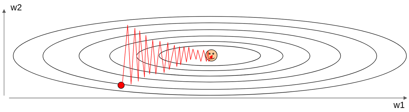
Consider a scenario where our loss function landscape looks like this: a long, narrow valley, or a ravine. The ellipses here represent level sets of the loss function, and the smiley face is at the minimum we want to reach. The question is: What if the loss changes quickly in one direction and slowly in another? For example, along the w2 direction (vertically), the valley is very steep – the loss changes rapidly. But along the w1 direction (horizontally), the valley is very shallow and elongated – the loss changes slowly. If we start at the red dot and apply standard SGD, what will happen? What gradient descent does is it always points in the direction of steepest descent. In such a ravine, the steepest direction is mostly perpendicular to the valley floor, pointing across the steep walls. So, SGD will tend to take large steps that oscillate back and forth across the narrow valley (the w2 direction, where the gradient is large). Because of these large oscillations, if we use a single learning rate, it has to be small enough to prevent divergence in this steep direction. However, this small learning rate means that progress along the shallow direction of the valley (the w1 direction, where the gradient component is small) will be agonizingly slow. The result is very slow progress along the shallow dimension, and a lot of jitter or oscillation along the steep direction, as shown by the red zigzag path. We’re making very inefficient progress towards the true minimum. This kind of behavior is characteristic of loss functions that are ill-conditioned.

Problem #2 with SGD: Local Minima and Saddle Points

The loss functions for deep neural networks are highly non-convex. This means they can have many local minima – points where the loss is lower than all its immediate neighbors, but not necessarily the global minimum (the lowest possible loss overall). They can also have saddle points.

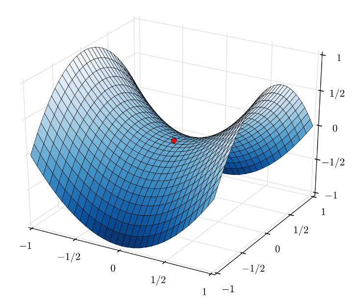
Saddle point, image source: https://en.wikipedia.org/wiki/Saddle_point

At a local minimum, or at a saddle point, the gradient is zero (or very close to zero). If the gradient is zero, then weights_grad in our update rule weights += - step_size * weights_grad is zero. This means the weights stop updating. Gradient descent gets stuck! It thinks it has found the bottom of a valley, but it might just be a small dip, or a point that’s flat in some directions but goes up in others.

Now, for a long time, people were very concerned about local minima being a major impediment to training deep networks. The fear was that SGD would get trapped in a poor local minimum and never find a good solution. However, more recent research, like the paper by Dauphin et al. (2014) cited here, suggests that in very high-dimensional spaces (which is where our weight matrices W live), saddle points are actually much more common than local minima. For a point to be a local minimum, the loss function needs to curve upwards in all dimensions around that point. For it to be a local maximum, it needs to curve downwards in all dimensions. For it to be a saddle point, it needs to curve upwards in some dimensions and downwards in others. In high dimensions, it’s statistically much more likely to have a mix of curvatures than for all curvatures to go in the same direction. So, while getting stuck is a problem, it’s often saddle points, rather than bad local minima, that are the primary culprits for slowing down or halting SGD. At a saddle point, the gradient is zero, but it’s not a minimum.

So, that’s the second major issue: points with zero or near-zero gradient (local minima and, more commonly, saddle points) can trap or significantly slow down SGD.

Problem #3 with SGD: Noisy Gradients

This problem is inherent in the “S” of SGD – the stochasticity. As we discussed, our loss \(L(W)\) is an average over all \(N\) training examples (plus regularization, which we’ll ignore for this point for simplicity). And it’s true gradient is:

\[ \nabla_W L = \frac{1}{N} \sum_{i = 1}^N \nabla_W L_i(x_i, y_i, W) \]

However, with minibatch SGD, we don’t compute this full sum. We compute the gradient on a small minibatch. This minibatch gradient is an estimate of the true gradient. Because the minibatch is a random sample, this estimate will be noisy. It won’t point exactly in the direction of the true steepest descent. If you take many different minibatches at the same point \(W\), you’ll get slightly different gradient vectors.

The noisy gradients mean that our steps won’t be as smooth as the idealized animation we saw earlier. They’ll be a bit erratic. While this noise can sometimes be helpful (e.g., for escaping sharp local minima or some saddle points), it also means that the convergence path can be jittery, and finding the exact minimum can be harder. The optimization path might dance around the minimum without settling perfectly.

So, these three problems – ill-conditioned landscapes (ravines), local minima/saddle points, and noisy gradients – are key challenges that standard SGD faces. This has motivated the development of more advanced optimization algorithms that try to mitigate these issues. One of the first and most important enhancements is the idea of momentum.

Momentum

The first major improvement we’ll discuss is adding Momentum to SGD. If SGD gets to a flat region where the gradient is zero, it stops. Momentum, like a ball rolling downhill, has inertia. It might be able to “roll through” small local minima or flat regions of saddle points because it has built up speed from previous gradients. In that zigzagging scenario, the gradient components across the ravine tend to cancel out on average over iterations due to the oscillation. However, the small gradient components along the valley consistently point in the same direction. Momentum helps to average out these oscillations and amplify the consistent movement along the valley floor. You can see the blue line (SGD+Momentum) makes much more direct progress towards the minimum compared to the black zigzagging SGD line. The noise in minibatch gradients causes SGD to jitter. Momentum helps to smooth out these noisy updates by taking a running average of the gradients. This leads to a more stable and often faster convergence towards the minimum

Now, for SGD + Momentum. The key idea is to continue moving in the general direction as the previous iterations. We introduce a “velocity” term, v, which accumulates a running mean of the gradients.

\[ \begin{align} v_{t+1} &= \rho v_t + \nabla f(x_t) \\ x_{t+1} &= x_t - \alpha v_{t+1} \end{align} \]

\(v_{t}\) is the velocity vector from the previous step. It’s initialized to zero.
\(\rho\) is the momentum coefficient (or friction term). It’s typically a value like 0.9 or 0.99. It determines how much of the previous velocity is retained. If ρ=0, we recover standard SGD (almost, as we’ll see the learning rate is applied differently).
In the first equation, we update the velocity: we take the old velocity \(v_t\), scale it down by \(\rho\), and then add the current gradient \(\nabla f(x_t)\). So, the velocity v is essentially an exponentially decaying moving average of the past gradients.
In the second equation, we update the parameters \(x\) by taking a step in the direction of this new velocity \(v_t+1\), scaled by the learning rate \(\alpha\). Crucially, we are now stepping with the velocity, not directly with the current gradient.

The intuition is that we build up “velocity” as a running mean of gradients. If gradients consistently point in the same direction, the velocity in that direction grows. If gradients oscillate, those components of the velocity tend to be dampened. The term \(\rho\) acts like friction. If \(\rho\) is close to 1 (e.g., 0.99), we have high momentum, and the velocity persists for a long time. If \(\rho\) is smaller (e.g., 0.5), it’s like having more friction, and the velocity relies more on recent gradients. The paper by Sutskever et al. (2013) is a classic reference highlighting the importance of momentum in deep learning

Here’s how this might look in code:

vx = 0 # initialize velocity to zero
while True:
  dx = compute_gradient(x) # current gradient
  vx = rho * vx + dx       # update velocity
  x -= learning_rate + vx  # update parameters

Momentum is a very powerful and widely used technique. But it’s not the only improvement over vanilla SGD. Other methods try to adapt the learning rate on a per-parameter basis, which can be particularly helpful for those ill-conditioned ravine-like loss surfaces.

Smarter steps with adaptive optimizer

Okay, so SGD with Momentum helps to accelerate in consistent directions and dampen oscillations. But what about that problem of different curvatures in different dimensions – the ravines? Momentum helps, but can we do even better? This leads us to optimizers that try to adapt the learning rate on a per-parameter basis. One popular example is RMSProp. Recall SGD+Momentum: we compute a velocity vx and update x using learning_rate * vx. Now, for RMSProp, developed by Tieleman and Hinton:

1grad_square = 0
while True:
  dx = compute_gradient(x)
2  grad_square = decay_rate * grad_square + (1 - decay_rate) * dx * dx
3  x -= learning_rate * dx / (np.sqrt(grad_squared) + 1e-7)

1: We maintain a variable grad_squared. This variable will keep track of an exponentially decaying average of the squared gradients for each parameter. It’s initialized to zero.
2: This is an exponentially weighted moving average. decay_rate is a hyperparameter, typically something like 0.9 or 0.99. We’re taking the previous grad_squared, decaying it, and adding the newly computed dx * dx (element-wise square of the current gradient), scaled by 1 - decay_rate. So, grad_squared accumulates information about the typical magnitude of recent gradients for each parameter.
3: this is the parameter update rule, we take our square root of our accumulated grad_squared this gives us something like the Root Mean Square of recent gradients, add a small epsilon (like 1e-7) for numerical stability to prevent division by zero if grad_squared is tiny, and then we divide the current gradient dx by this term.

The effect of this division by np.sqrt(grad_squared) is crucial. If a particular parameter has consistently had large gradients in the past (meaning its corresponding element in grad_squared is large), then np.sqrt(grad_squared) will be large, and the effective step size for that parameter learning_rate / (np.sqrt(grad_squared) + epsilon) will be smaller. Conversely, if a parameter has consistently had small gradients (so grad_squared for it is small), then np.sqrt(grad_squared) will be small, and its effective step size will be larger. This effectively gives us per-parameter learning rates or adaptive learning rates. The learning rate is adapted for each parameter based on the history of its gradient magnitudes.

What happens with RMSProp? Specifically, how does this help with that ravine problem? What happens is that progress along “steep” directions is damped, and progress along “flat” directions is accelerated. Think back to our ravie. In the steep direction (e.g., w2), the gradients dx are large. This means dx * dx will be large, and grad_squared will accumulate to a large value for that dimension. Consequently, when we divide dx by np.sqrt(grad_squared), we significantly reduce the step size in that steep direction. This helps to prevent the oscillations. In the flat, shallow direction (e.g., w1), the gradients dx are small. dx * dx will be small, and grad_squared will be small for that dimension. When we divide dx by a small np.sqrt(grad_squared), the effective step size for that direction is relatively larger (or at least not as suppressed). This helps to make faster progress along the shallow valley. So, RMSProp automatically adjusts the learning rate for each parameter, making bigger steps in directions where gradients have been small and smaller steps in directions where gradients have been large.

blue line: RMSProp, red line: SGD+Momentum, black line: SGD

RMSProp is a very effective optimizer and was a popular choice for quite some time. It directly addresses the issue of different learning rates being needed for different parameter dimensions. Now, what if we could combine the benefits of momentum with the adaptive learning rates of RMSProp? That leads us to Adam.

Here’s a look at the core of the Adam optimizer, presented as “Adam (almost)” because it’s missing one small but important detail we’ll get to. This was introduced by Kingma and Ba in their 2015 ICLR paper.

first_moment = 0
second_moment = 0
while True:
  dx = compute_gradient(x)
1  first_moment = beta1 * first_moment + (1 - beta1) * dx
2  second_moment = beta2 * second_moment + (1 - beta2) * dx * dx
3  x -= learning_rate * first_moment / (np.sqrt(second_moment) + 1e-7)

1: This is an exponentially decaying moving average of the gradient itself. beta1 is a decay rate (e.g., 0.9). This looks very much like the velocity update in SGD+Momentum! It’s capturing the “momentum” aspect which is an estimate of the mean of the gradients.
2: This is an exponentially decaying moving average of the squared gradients. beta2 is another decay rate (e.g., 0.999). This looks exactly like the grad_squared update in RMSProp! It’s capturing information about the variance (or uncentered second moment) of the gradients.
3: Here, we’re using the first_moment (our momentum term) in the numerator, and we’re dividing by the square root of the second_moment (our RMSProp-like adaptive scaling term) in the denominator.

It’s sort of like RMSProp with momentum. It’s trying to get the best of both worlds: the acceleration benefits of momentum and the per-parameter adaptive learning rates. Remember, first_moment and second_moment are initialized to zero. What’s the implication of this?

At the very first timestep (and for the first few timesteps), because first_moment and second_moment start at zero and the decay rates beta1 and beta2 are typically close to 1 (e.g., 0.9, 0.999), these moving average estimates will be biased towards zero. They haven’t had enough gradient information to “warm up” to their true values. This can cause the initial steps to be undesirably small. This is where the “almost” part is resolved. The full form of Adam includes a bias correction step to address this initialization bias.

first_moment = 0
second_moment = 0
for t in range(1, num_iterations): # t is the timestep
  dx = compute_gradient(x)
  first_moment = beta1 * first_moment + (1 - beta1) * dx
  second_moment = beta2 * second_moment + (1 - beta2) * dx * dx

  # Bias correction
  first_unbias = first_moment / (1 - beta1**t)
  second_unbias = second_moment / (1 - beta2**t)

  x -= learning_rate * first_unbias / (np.sqrt(second_unbias) + 1e-7)

Here t is the current iteration number (timestep). At the beginning with small t, beta1**t and beta2**t are close to beta1 and beta2. So, (1 - beta1**t) and (1 - beta2**t) are small numbers, which effectively scales up the first_moment and second_moment estimates, counteracting their initial bias towards zero. As t gets large, beta1**t and beta2**t approach zero (since beta1, beta2 < 1), so (1 - beta1**t) and (1 - beta2**t) approach 1, and the bias correction has less and less effect. The parameter update then uses these bias-corrected first_unbias and second_unbias estimates. This bias correction is for the fact that the first and second moment estimates start at zero and would otherwise be biased, especially during the early stages of training.

blue line: RMSProp, red line: SGD+Momentum, black line: SGD, purple: Adam

The Adam optimizer, with its combination of momentum-like behavior and RMSProp-like adaptive scaling, plus this bias correction, has proven to be very effective and robust across a wide range of deep learning tasks and architectures. The original paper suggests default values for the hyperparameters:

beta1 = 0.9 (for the first moment/momentum)
beta2 = 0.999 (for the second moment/RMSProp-like scaling)
learning_rate typically in the range of 1e-3 (0.001) or 5e-4 (0.0005).
The epsilon for numerical stability is often 1e-7 or 1e-8.

And indeed, Adam with these default settings (beta1=0.9, beta2=0.999, and a learning_rate like 1e-3) is often a great starting point for many models! It’s frequently the first optimizer people try, and it often works quite well out of the box without extensive hyperparameter tuning, though tuning the learning rate is still important. Adam is a fantastic general-purpose optimizer. However, like all things, it’s not perfect, and some subtleties have emerged, particularly regarding how it interacts with weight decay (L2 regularization).

This leads us to AdamW: an Adam Variant with Weight Decay. The question to consider is: How does regularization interact with the optimizer? (e.g., L2)

Remember that our full loss function is typically \(L_{data} + \lambda R(W)\). If \(R(W)\) is L2 regularization, then its gradient is \(2\lambda W.\) This gradient of the regularization term gets added to the gradient of the data loss term to form the total dx = compute_gradient(x). So, how does this interaction play out with an adaptive optimizer like Adam? The answer, perhaps unsurprisingly, is: It depends! Specifically, it depends on how the L2 regularization (weight decay) is implemented with respect to the adaptive learning rate mechanism. In Standard Adam (and many other adaptive gradient methods like RMSProp or AdaGrad), the L2 regularization term \(\lambda W\) is typically added to the gradient of the data loss before the moment calculations. So, dx = gradient_of_data_loss + gradient_of_L2_regularization. This combined dx is then used during the moment calculations (for first_moment and second_moment). What this means is that the L2 regularization gradient gets scaled by the adaptive learning rates (the 1/sqrt(second_moment) term). If second_moment is large for a particular weight (meaning its gradients have been large), then the effective weight decay for that parameter is also reduced. This coupling means that the strength of the weight decay is not uniform and can be different for different parameters, and can change over time in a way that might not be optimal. Larger gradients lead to smaller effective weight decay.

AdamW introduced by Loshchilov and Hutter, 2017, in “Decoupled Weight Decay Regularization” proposes a different approach. Instead of adding the L2 regularization gradient into dx before the moment calculations, AdamW performs weight decay after the moment updates, directly on the weights themselves. So, the first_moment and second_moment are computed using only the gradient of the data loss. Then, the weight decay is applied as a separate step, effectively by subtracting learning_rate * weight_decay_coefficient * weights from the weights after the Adam step that uses first_unbias and second_unbias. So, AdamW is now often preferred over standard Adam when L2 regularization is used, as it implements weight decay in a way that is often more effective and closer to its original intention. Many deep learning libraries now offer AdamW as a distinct optimizer.

Learning rate schedules

Now, let’s turn our attention to a hyperparameter that is critical for all of them: the learning rate, often referred to as step_size. In the vanilla gradient descent update, weights += - step_size * weights_grad, the learning rate determines how big of a step we take in the negative gradient direction. All the optimizers we’ve discussed – SGD, SGD+Momentum, RMSProp, Adam, AdamW all have the learning rate as a crucial hyperparameter. Choosing the right learning rate is often one of the most important parts of getting good performance from a deep learning model.

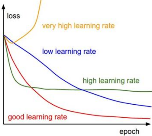
So, the question is: Which one of these learning rates is best to use? Is there a single magic value? The answer is: In reality, all of these could be good learning rates… at different stages of training. This is a key insight. A single, fixed learning rate throughout the entire training process might not be optimal. Early in training, when you’re far from a good solution, a relatively larger learning rate can help you make rapid progress across the loss landscape. However, as you get closer to a minimum, that same large learning rate might cause you to overshoot and bounce around the minimum, preventing you from settling into the very bottom of the valley. In this later stage, a smaller learning rate is often beneficial to fine-tune the weights and converge more precisely. This idea that the optimal learning rate might change during training leads directly to the concept of learning rate schedules, also known as learning rate decay. We don’t just pick one learning rate and stick with it; we dynamically adjust it as training progresses.

One common strategy is Step Decay.

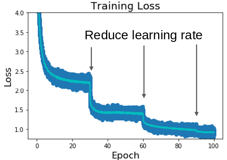
training loss epoch, notice the distinct drops in loss at certain epochs

The strategy here is to reduce the learning rate at a few fixed points during training. For example, a common schedule for training ResNets on ImageNet is to start with a certain learning rate, and then multiply it by 0.1 after, say, 30 epochs, then again by 0.1 after 60 epochs, and perhaps one more time after 90 epochs. You can see that after the learning rate is reduced (indicated by the arrows), the loss often plateaus for a bit and then finds a new, lower level. This happens because with a smaller learning rate, the optimizer can more finely navigate the bottom of the loss valley it has reached

Step decay is quite effective, but it requires choosing when to drop the learning rate and by how much. Are there smoother ways to decay the learning rate? Yes! Another very popular schedule is Cosine Decay.

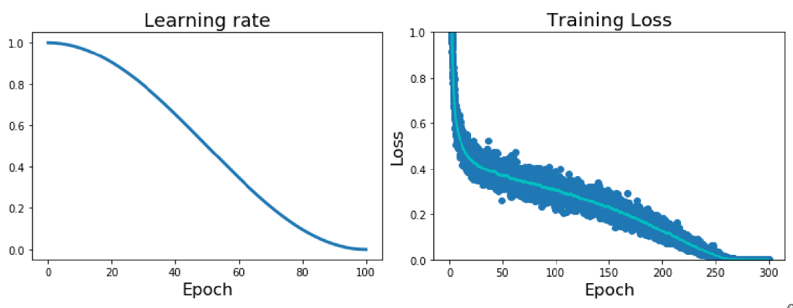
The formula is:

\[ \alpha_t = \frac{1}{2} \alpha_0 \left(1 + \cos\left(\frac{t}{T} \pi\right)\right) \]

Where:

\(\alpha_0\) is initial learning rate
\(\alpha_t\) is the learning rate at epoch \(t\)
\(T\) is the total number of epochs you plan to train for

The plot shows how this learning rate evolves over epochs. It starts at \(\alpha_0\) and smoothly decreases, following a cosine curve, until it reaches near zero at the end of training (epoch \(T\)). This smooth decay is often found to work very well in practice and is less sensitive to the exact choice of drop points compared to step decay. Many recent state-of-the-art models use cosine annealing, sometimes with warm restarts which we’re not covering in detail here but involves periodically resetting the learning rate and re-annealing, as in the Loshchilov and Hutter paper. And on the right is an example of what the training loss might look like when using a cosine decay schedule. You see a generally smooth decrease in loss over a larger number of epochs, without the sharp drops associated with step decay. It just gradually refines the solution as the learning rate smoothly anneals.

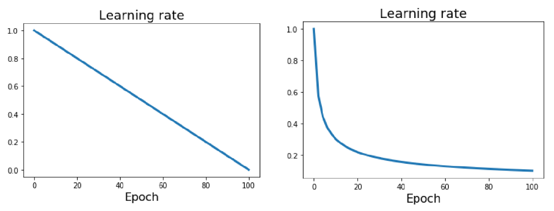
left: Linear Decay, right: Inverse Square Root Decay

Another simple schedule is Linear Decay, the formula is:

\[ \alpha_t = \alpha_0 (1 - \frac{t}{T}) \]

The learning rate decreases linearly from \(\alpha_0\) down to 0 over \(T\) epochs. This is also a common choice, used in famous models like BERT, for example. The plot shows this straight-line decrease.

And one more example: Inverse Square Root Decay. The formula is:

\[ \alpha_t = \frac{\alpha_0}{\sqrt{t}} \]

The learning rate decreases proportionally to the inverse square root of the epoch number \(t\). This schedule makes the learning rate drop relatively quickly at the beginning and then more slowly later on. This was famously used in the original “Attention is All You Need” Transformer paper.

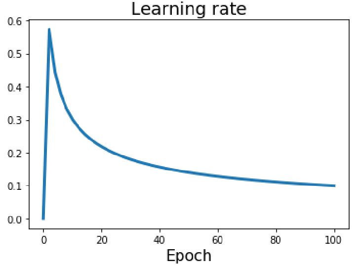
There’s one more important trick related to learning rates, especially when using large initial learning rates or large batch sizes: Linear Warmup. The idea is that high initial learning rates can sometimes make the loss explode right at the beginning of training, especially if the initial weights are far from good and produce very large gradients. The model can become unstable. To prevent this, a common practice is to linearly increase the learning rate from 0 (or a very small value) up to your target initial learning rate \(\alpha_0\) over the first few thousand iterations (e.g., the first ~5,000 iterations or the first epoch). The plot shows this: the learning rate starts at 0, ramps up linearly to a peak (this is our \(\alpha_0\)), and then a decay schedule like cosine or step takes over. This “warmup” phase allows the model to stabilize a bit with small updates before the more aggressive learning rate kicks in. It’s a very common and effective technique, particularly in training large models like Transformers. There’s also an interesting empirical rule of thumb often cited (e.g., from Goyal et al.’s paper “Accurate, Large Minibatch SGD”): If you increase the batch size by N, you should also scale the initial learning rate by N (or \(\sqrt{N}\) in some cases), often in conjunction with a warmup. The intuition is that larger batches give more stable gradient estimates, so you can afford to take larger steps.

So, managing the learning rate is not just about picking a single value, but often about defining a schedule that includes an initial phase (like warmup) and a decay phase. This is a critical part of the “art” of training deep neural networks.

So, in practice:

Adam(W) is a good default choice in many cases. It often works reasonably well even with a constant learning rate (though a schedule is still generally better) and requires less manual tuning of the learning rate compared to SGD with momentum. AdamW is preferred if you’re using L2 regularization.
SGD+Momentum can outperform Adam but may require more tuning of the learning rate and its schedule. There’s a bit of an ongoing debate and empirical evidence suggesting that with careful tuning, SGD+Momentum can sometimes find solutions that generalize better than those found by Adam, especially for certain types of vision models. However, “careful tuning” is the operative phrase.