Neural network and backpropagation

Deep learning today

“Deep learning” this is the term you hear everywhere now, and it’s really transformed not just computer vision, but many areas of artificial intelligence. And the progress, especially in the last few years, has been absolutely outstanding. Let’s just take a moment to appreciate some of the incredible capabilities that deep learning models have unlocked, particularly in the realm of image generation and understanding.

Images generated by DALL-E 2 on Sam Altman tweet and https://openai.com/dall-e-2/

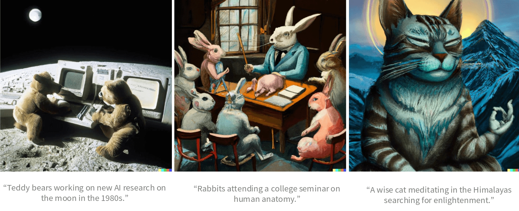
These images are generated by DALL-E 2. These are not photographs; they are synthesized by an AI from text prompts. The level of detail, the coherence of the scenes, and the creativity are just remarkable. These models are clearly understanding complex relationships between concepts and visual elements. In 2022 Ramesh et al. released “Hierarchical Text-Conditional Image Generation with CLIP Latents” give us a glimpse into how some of these text-to-image models work. So basically it involves an image encoder, a text encoder, a prior model that learns to associate these representations, and then a decoder to generate the image, the CLIP objective, which learns joint embeddings of images and text, plays a crucial role here.

Images from “Improving image generation with better captions” paper (2023)

More recently, we’ve seen DALL-E 3. These models are getting exceptionally good at interpreting nuanced textual descriptions. Notice the image on the right, the model not only generates the individual elements but also composes them into a coherent scene with multiple interacting characters, and it even captures the specified “graphic novel” style. You can see how it even annotates which parts of the image correspond to which parts of the prompt.

Thinking with images (image from https://openai.com/index/introducing-o3-and-o4-mini/)

This isn’t just about image generation. Now with o3 and o4 mini, these model can integrate images directly into their chain of thought which they call “Visual reasoning in action”, they can reason, think about the image. This shows a deep level of visual reasoning.

Thinking with images allows you to interact with ChatGPT more easily. You can ask questions by taking a photo without worrying about the positioning of objects, whether the text is upside down or there are multiple physics problems in one photo. Even if objects are not obvious at first glance, visual reasoning allows the model to zoom in to see more clearly.

Segment Anything Model (SAM)

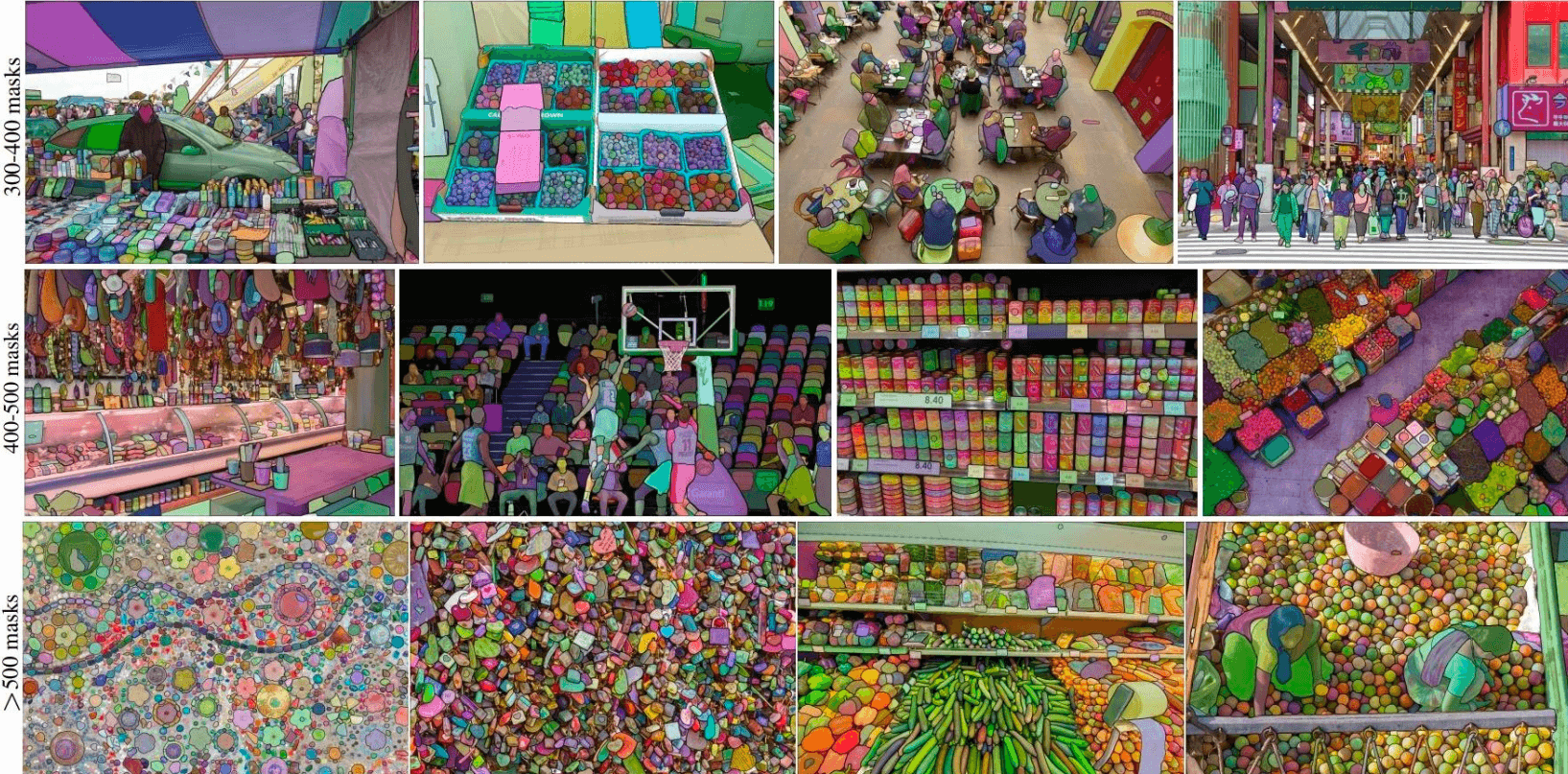
We also have models like the Segment Anything Model (SAM). SAM is remarkable because it can generate segmentation masks for any object in an image, just from a prompt or a click. Look at the density of masks it can produce, it can segment hundreds, even thousands of objects and parts of objects within a single image. This has huge implications for image editing, robotics, and a wide range of computer vision tasks.

And then we move into video. This is an example from Sora, a recent model from OpenAI that generates video from text. The quality, coherence over time, and realism are truly groundbreaking. Sora can do things like animating images that were themselves generated by models like DALL-E. It can also do video-to-video editing, where you provide an input video and a text prompt, and it modifies the video accordingly. The model understands the content of the video and can plausibly alter its style or elements based on text.

Base compute

4x compute

32x compute

And a key theme, as with many of these large generative models, is the impact of more compute. These video show the output of Sora for the same prompt, but with increasing amounts of compute used for generation. You can clearly see how the quality, detail, and realism improve significantly as more computational resources are applied. This scaling hypothesis that bigger models and more data, trained with more compute, lead to better performance has been a driving force in deep learning.

So, these examples are just a taste of what deep learning is achieving. It’s creating tools that can understand, generate, and manipulate visual information in ways that were science fiction just a decade ago. The common thread underlying all these incredible advancements is the use of neural networks, often very deep ones, trained on massive datasets. And that’s what we’re here to understand today: what are these neural networks, and how do we train them?

What is neural network?

We’re going to build these up step-by-step. And perhaps surprisingly, we’ll start with something very familiar. Think about our original linear classifier. Before, when we talked about linear score functions, we had this simple equation: \(f(x) = Wx\). Here \(x\) is our input vector, say an image flattened into a D-dimensional vector so \(x\) is in \(\mathbb{R}^D\). And \(W\) is our weight matrix, of size C x D, where C is the number of classes. This matrix \(W\) projects our D-dimensional input into a C-dimensional space of class scores. This is the simplest possible “network” if you like - a single linear layer. Now, how do we make this more powerful? How do we build a neural network with, say, 2 layers? We take our original linear score function, \(Wx\), and we are going to insert something in the middle. Now our new equation look like this:

\[ f(x) = W_2 \max(0, W_1x) \]

We’re still starting with our input \(x\). We first multiply it by a weight matrix, let’s call it \(W_1\). So we compute \(W_1x\). If x is \(\mathbb{R}^D\), then \(W_1\) will be a matrix of size H x D. H here represents the number of neurons or hidden units in this first layer. So, \(W_1x\) gives us an H-dimensional vector. Then we apply a non-linear function. Here we’re using \(max(0, ...)\) which we will talk about this for a moment. The output of this non-linearity is now an H dimensional vector, we then multiply this vector by a second weight matrix, \(W_2\). This \(W_2\) matrix will have dimensions C x H, where C is still our number of output classes. So, \(W_2\) takes the H-dimensional output of the first layer and maps it down to our C class scores. In practice we will usually add a learnable bias at each layer as well. So, more accurately, the operations would look like \(W_1x + b_1\) and \(W_2h + b_2\) (where h is the output of the first layer). We often absorb the bias into the weight matrix by augmenting \(x\) with a constant 1, as we’ve discussed before, or handle it as a separate bias vector. For now, we’ll keep the notation a bit cleaner by omitting explicit biases, but remember they’re typically there.

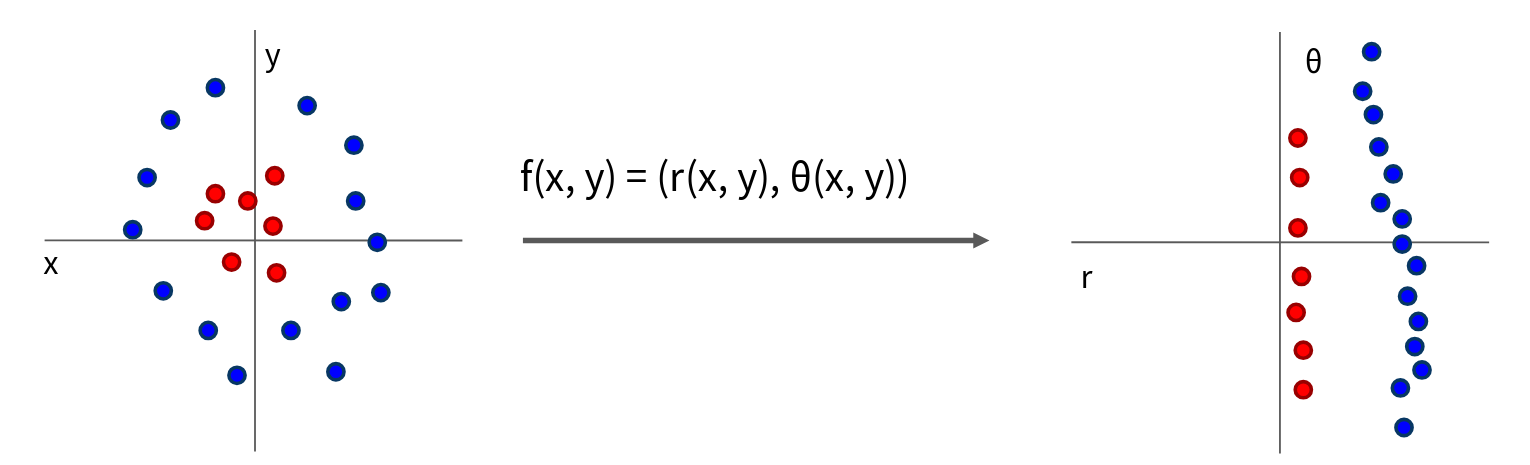
Consider this example, We have some data points in a 2D space. The red points form a cluster in the center, and the blue points surround them. Can we separate these red and blue points with a linear classifier? No, you can’t draw a single straight line in this x, y space that perfectly separates the red from the blue. A linear classifier, by definition, can only learn linear decision boundaries. But what if we could transform our input space? This is where the idea of feature transformations comes in, and it’s closely related to what neural networks do. Imagine we apply a function \(f(x, y)\) that maps our original Cartesian coordinates (x, y) to polar coordinates (\(r(x,y)\), \(\theta(x,y)\)). So, \(r\) is the radius from the origin, and \(\theta\) is the angle. Now in this new \((r, \theta)\) space, shown on the right. The red points, which were close to the origin, now have small \(r\) values. The blue points, which were further out, now have larger \(r\) values. In this transformed space, the red and blue points are linearly separable! We can now draw a simple horizontal line (a constant \(r\) value) that separates them.

This is the core idea. The non-linearities in a neural network allow the network to learn these kinds of powerful feature transformations. The first layer \(W_1x\) followed by the \(\max(0, ...)\) non-linearity effectively computes a new representation of the input. And then the next layer \(W_2\) operates on this transformed representation. By stacking these layers with non-linearities, the network can learn increasingly complex and abstract features that make the original problem (like classification) easier, often making it linearly separable in some high-dimensional learned feature space.

Neural network architectures

You’ll hear these kinds of networks, \(f = W_2 \max(0, W_1x)\), referred to by a few names. While “Neural Network” is a very broad term, the specific architecture we’re discussing here is often more accurately called a “fully-connected network”. This is because, as we’ll see when we visualize them, every neuron (or unit) in one layer is connected to every neuron in the subsequent layer. Another term you might encounter, especially in older literature, is “multi-layer perceptron” or MLP. For our purposes, when we talk about a basic neural network with these stacked layers of matrix multiplies and non-linearities, we’re generally talking about a fully-connected network. And remember, we usually add learnable biases at each layer.

Now, there’s nothing stopping us from making these networks deeper. We can extend this to 3 layers, or indeed many more. Our 2-layer network was \(f = W_2 \max(0, W_1x)\). A 3-layer neural network simply inserts another layer of weights and non-linearity:

\[ \begin{align} f &= W_3 \max(0, W_2 \max(0, W_1x)) \\ x &\in \mathbb{R}^D, W_1 \in \mathbb{R}^{H_1 \times D}, W_2 \in \mathbb{R}^{H_2 \times H_1}, W_3 \in \mathbb{R}^{C \times H_2} \end{align} \]

A quick note on terminology: when we say an “N-layer neural network,” we typically mean a network with N layers of weights, or N-1 hidden layers plus an output layer. So, our 2-layer Neural Network here has one hidden layer (the W_1 transformation produces its activations), and our 3-layer Neural Network has two hidden layers (activations produced after \(W_1\) and after \(W_2\)). The input is sometimes called the input layer, but it doesn’t usually involve learnable weights or non-linearities in the same way.

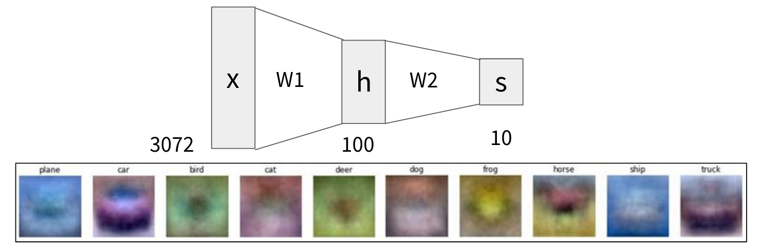
We can visualize this as a form of hierarchical computation. So what’s the advantage of this hidden layer h? Think back to our linear classifier, \(f = Wx\). Each row of \(W\) could be interpreted as a “template” for one of the classes. For CIFAR-10, we’d learn 10 templates. Now, with a 2-layer neural network, the first weight matrix W_1 (e.g., 100x3072) can be thought of as learning many more templates – in this example, 100 templates. These aren’t necessarily templates for the final classes directly. Instead, they are like intermediate features or visual primitives. The hidden layer \(h\) then represents the extent to which each of these 100 learned “templates” or features is present in the input image. Then, the second weight matrix \(W_2\) (10x100) learns how to combine these 100 intermediate features to produce the final scores for the 10 classes. So, instead of learning just 10 direct templates, we learn, say, 100 more foundational templates, and these templates can be shared and re-weighted by W_2 to form the decision for each class. This gives the network much more flexibility and expressive power. It can learn a richer set of features and then learn complex combinations of those features.

Activation functions

Now, a key question arises from this construction, why do we want non-linearity? Let’s consider the function we just built: \(f = W_2 \max(0, W_1x)\). What if we didn’t have that \(\max(0, ...)\) non-linearity? What if our function was just \(f = W_2 W_1 x\)? Well, if \(W_1\) is a matrix and \(W_2\) is a matrix, then their product, \(W_2 W_1\), is just another matrix. Let’s call it \(W_{prime}\). So, \(f = W_{prime} x\). This is just a linear classifier again! Stacking multiple linear transformations without any non-linearity in between doesn’t actually increase the expressive power of our model beyond a single linear transformation. It collapses back down to a linear function. The non-linearity is what allows us to learn much more complex functions. So, what are some common choices for these activation functions?

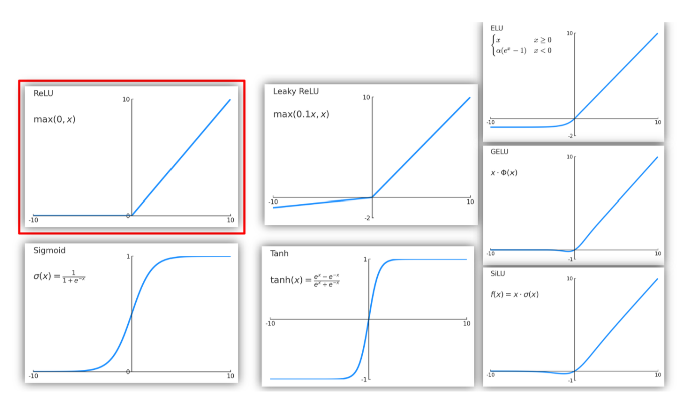
The one we’ve been using, \(\max(0, x)\), is called ReLU (Rectified Linear Unit), and you can see its plot in the top left, highlighted in red. For any negative input, it outputs zero. For any positive input, it outputs the input itself. It’s simple, computationally efficient, and works remarkably well in practice. In fact, ReLU is a good default choice for most problems and is very widely used. But there are many other activation functions people have explored like Leaky ReLU This can sometimes help with issues where ReLU units “die” or Sigmoid This function squashes its input into the range (0, 1). It was historically very popular, especially in the early days of neural networks, because its output can be interpreted as a probability or a firing rate of a neuron. However, it suffers from vanishing gradients for very large positive or negative inputs, which can slow down learning in deep networks. Tanh this function squashes its input into the range (-1, 1). It’s zero-centered, which can sometimes be advantageous over sigmoid. Like sigmoid, it also suffers from vanishing gradients at the extremes. And a lot of ReLU variations like ELU, GELU, SiLU, or what ever it is just ending with LU. But you shouldn’t expect much from those activation functions, you might get a slightly better result when using this activation function over one another depend on the problem you’re trying to solve, but trust me just stick with ReLU and it will work pretty much with most of the problems you might come up with.

A note on network size and regularization

Okay, so we have these building blocks: layers composed of a linear transformation followed by a non-linear activation function. Now, let’s think about how we arrange these layers to form different neural network architectures.

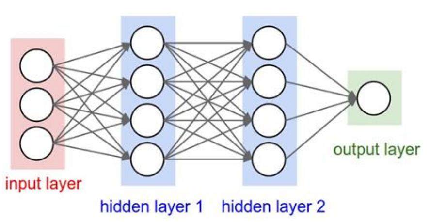
You’ll often see neural networks visualized like this, with nodes and connections. We have a “3-layer Neural Net” or a “2-hidden-layer Neural Net”. The circles on the far left represent the input layer – these are just our raw input features, say the pixel values of an image. The next set of circles in the middle is the hidden layer. Each unit here computes a weighted sum of the inputs, adds a bias, and then passes it through an activation function (like ReLU). And finally, the circles on the right form the output layer, which produces our final class scores, or perhaps a regression value. The output of the first hidden layer becomes the input to the second hidden layer, which then feeds into the output layer. The key thing to notice in these diagrams are the lines connecting the nodes. These layers are typically Fully-connected layers. This means that every neuron in the input layer is connected to every neuron in the first hidden layer. And every neuron in the first hidden layer is connected to every neuron in the second hidden layer, and so on, up to the output layer. Each of these connections has an associated weight.

So, when we say an N-layer Neural Net, we generally mean there are N layers of weights and N layers of activations being computed or N-1 hidden layers plus an output layer. The input itself isn’t usually counted as a layer in this sense, as it doesn’t perform a computation with learnable weights. Let’s look at an example feed-forward computation for a neural network, to make this more concrete.

1f = lambda x: 1.0/(1.0 + np.exp(-x))
2x = np.random.randn(3, 1)
3h1 = f(np.dot(W1, x) + b1)
4h2 = f(np.dot(W2, h1) + b2)
5out = np.dot(W3, h2) + b3

1

we define our activation function f. In this example, they’re using a sigmoid

2

we have some input x, which is a 3x1 vector.

3

get the activations of the first hidden layer, h1. W_1would be a 4x3 weight matrix, and b1 would be a 4x1 bias vector then we performs the matrix multiplication and add the bias b1. Finally we apply the activation function f element-wise to the result. So h1 will be a 4x1 vector.

4

similarly, for the second hidden layer activations, h2

5

finally for the output neuron, out, W3 would be a 1x4 matrix b3 a 1x1 bias. Notice that for the output layer, an activation function isn’t always applied, or a different one might be used depending on the task for example softmax for multi-class classification, sigmoid for binary classification, or no activation for regression.

This step-by-step process, from input to output, is called the forward pass. Now, it might seem like these networks are incredibly complex, but you might be surprised to learn that a full implementation of training a 2-layer Neural Network needs only about 20 lines of Python code using NumPy. This is, of course, a simplified example, but it captures all the essential components

import numpy as np
from numpy.random import rand

1N, D_in, H, D_out = 64, 1000, 100, 10
x, y = randn(N, D_in), randn(N, D_out)
w1, w2 = randn(D_in, H), randn(H, D_out)

2for t in range(2000):
  h = 1 / (1 + np.exp(-x.dot(w1)))
  y_pred = h.dot(w2)
  loss = np.square(y_pred - y).sum()
  print(t, loss)

3  grad_y_pred = 2.0 * (y_pred - y)
  grad_w2 = h.T.dot(grad_y_pred)
  grad_h = grad_y_pred.dot(w2.T)
  grad_w1 = x.T.dot(grad_h * h * (1 - h))

4  w1 -= 1e-4 * grad_w1
  w2 -= 1e-4 * grad_w2

1

we define the network, set up our hyperparameters. We then create some random input data X and target labels y, we initialize our weight matrices w1 and w2

2

next we perform forward pass

3

after the forward pass, we need to calculate the analytical gradients. This is the core of how we’ll update our weights. We’re essentially applying the chain rule to work backward from the loss and find how w1 and w2 affect that loss. We’ll dive much deeper into this process, called backpropagation, very soon.

4

And the final step in our training loop is to perform the gradient descent update. We simply take our current weights and subtract the gradient (multiplied by a small learning rate, here 1e-4) to move in the direction that reduces the loss.

And that’s it! In about 20 lines, we have a complete training procedure for a 2-layer neural network. Now, an obvious question that arises when designing these networks is how do we go about setting the number of layers and their sizes? This is a fundamental question in neural network design, and it relates to the “capacity” of the model

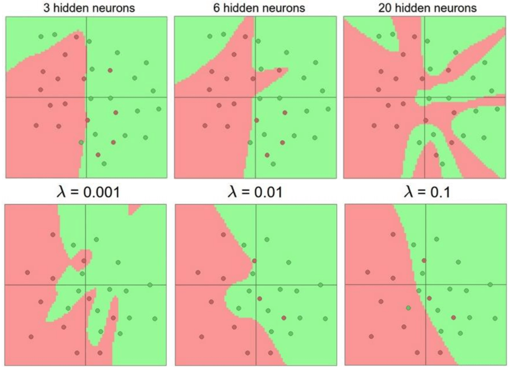
The diagrams in the first row illustrate the decision boundary learned by a two layer neural network with a varying number of neurons in its single hidden layer, trying to classify some 2D points. With only 3 hidden neurons, the network can learn a relatively simple decision boundary. When we increase to 6 hidden neurons, the network has more capacity. It can learn a more complex, wigglier decision boundary, fitting the data a bit better. And with 20 hidden neurons, it can learn an even more intricate boundary, potentially capturing finer details of the data distribution. The general principle here is that more neurons = more capacity. A network with more neurons (and more layers, which we’ll get to) can approximate more complex functions. It has more parameters, more knobs to turn, so it can fit more complicated patterns in the data. Now, if more neurons give more capacity, you might be tempted to think: “Great! I’ll just make my network huge, and it will fit the training data perfectly!”. But there’s a catch, and that’s overfitting. A network with too much capacity might learn the training data perfectly, including all its noise but fail to generalize to new and unseen data.

So how do we control this? One might think “Okay, I’ll just make my network smaller to prevent overfitting.” However, the general wisdom in the deep learning community now is: Do not use the size of the neural network as your primary regularizer. Use stronger regularization instead. What does this mean? It’s generally better to use a larger network that has the potential to learn the true underlying function well, and then control overfitting using explicit regularization techniques like L2 regularization, dropout, or data augmentation. Look at these plots at the bottom. They show the decision boundary for a network of a fixed, reasonably large size, but with different strengths of L2 regularization, controlled by \(\lambda\). The idea is that it’s often better to make your network “big enough” (in terms of layers and neurons) to have sufficient capacity to represent the complexity of the true underlying function, and then use regularization techniques to prevent it from merely memorizing the training data. Trying to find the “perfect” small size for your network is often harder and less effective than using a larger network with good regularization.

How to compute gradients?

Okay, so now we have our neural network, which is essentially a more complex, nonlinear score function. For a 2-layer network, our scores s are given by \(f(x; W_1, W_2) = W_2 \max(0, W_1x)\). This function takes our input x and our learnable parameters \(W_1\) and \(W_2\) and produces class scores. Once we have these scores, the rest of the framework we developed for linear classifiers still applies. We need a loss function to tell us how good these scores are. For example, we can use the Hinge Loss (or SVM loss) on these predictions:

\[ L_i = \sum_{j \neq y_i} \max(0, s_j - s_{y_i} + 1) \]

This is exactly the same hinge loss we saw before. It penalizes the network if the score \(s_j\) for an incorrect class \(j\) is not sufficiently lower than the score \(s_{y_i}\) for the correct class \(y_i\) (by a margin of 1). We could just as easily use the Softmax loss (cross-entropy loss) here. The choice of loss function depends on the specific problem and desired properties, just like with linear models. Next, we also typically include a regularization term to prevent overfitting. A common choice is L2 regularization: \(R(W) = \sum_k W_k^2\). This penalizes large values in our weight matrices.

And finally, the total loss \(L\) is the average of the data loss \(L_i\) over all N training examples, plus our regularization terms.

\[ L = \frac{1}{N} \sum_{i=1}^N L_i + \lambda R(W_1) + \lambda R(W_2) \]

Notice that now we have regularization terms for each of our weight matrices, \(W_1\) and \(W_2\) and if we had more layers, we’d regularize all their weights as well. The \(\lambda\) hyperparameter controls the strength of this regularization. So the overall structure is very familiar, 1) define a score function. 2) define a loss function. 3) add regularization. Our goal is still the same find the weight \(W_1\), \(W_2\) that minimize this total loss \(L\). But now, our score function f is more complex. It’s a nested composition of functions with matrix multiplies and non-linearities. This brings us to the next big challenge: How to compute gradients?

To use gradient descent, we need to compute the partial derivatives of the total loss \(L\) with respect to each of our parameters. That is, we need \(\frac{\partial L}{\partial W_1}, \frac{\partial L}{\partial W_2}\), if we can compute these gradients then we can update \(W_1\) and \(W_2\) using our standard gradient descent rule: \(W_1 = W_1 - learning\_rate \frac{\partial L}{\partial W_1}\), and similarly for \(W_2\). So how do we get these gradients? One idea which turns out to be a bad idea is to try and derive \(\frac{\partial L}{\partial W}\) on paper, analytically, and for the entire complex function. Think back to our linear classifier with SVM loss. Even for that relatively simple case, where \(s = f(x;W) = Wx\), and \(L_i = \sum \max(0, s_j - s_{y_i} + 1)\), deriving the full gradient \(\frac{\partial L}{\partial W}\) was already a bit involved. We had to expand it all out, as shown here, and then take derivatives.

\[ \begin{align} L_i &= \sum_{j \neq y_i} \max(0, s_j - s_{y_i} + 1) \\ &= \sum_{j \neq y_i} \max(0, W_{j,:} \cdot x + W_{y_i, :} \cdot x + 1) \\ L &= \frac{1}{N} \sum_{i=1}^N L_i + \lambda \sum_k W_k^2 \\ &= \frac{1}{N} \sum_{i=1}^N \sum_{j \neq y_i} \max(0, W_{j,:} \cdot x + W_{y_i, :} \cdot x + 1) + \lambda \sum_k W_k^2 \\ \nabla_W L &= \nabla_W \left(\frac{1}{N} \sum_{i=1}^N \sum_{j \neq y_i} \max(0, W_{j,:} \cdot x + W_{y_i, :} \cdot x + 1) + \lambda \sum_k W_k^2 \right) \end{align} \]

Now imagine doing this for our 2-layer neural network, where \(s\) itself is \(W_2 * \max(0, W_1 x)\). The expression for \(L\) in terms of the raw inputs \(x\) and weights \(W_1\), \(W_2\) would become much, much more complicated. It would be very tedious. It involves a lot of matrix calculus, and you’d need a lot of paper (or whiteboard space!). It’s very easy to make mistakes. What if we want to change our loss function? Say we initially derived everything for Hinge loss, and now we want to try Softmax loss. We’d have to re-derive everything from scratch! That’s not flexible at all. This approach is simply not feasible for very complex models. Modern deep neural networks can have tens, hundreds, or even thousands of layers, with various types of operations. Deriving the full analytical gradient for such a beast by hand is practically impossible and incredibly error-prone. So, we need a more systematic, more modular, and more scalable way to compute these gradients. And that leads us to a better idea: Computational graphs + Backpropagation.

The core idea here is to break down our complex function from input \(x\) and weights \(W\) all the way to the final loss \(L\) into a sequence of simpler, elementary operations. We can represent this sequence as a computational graph

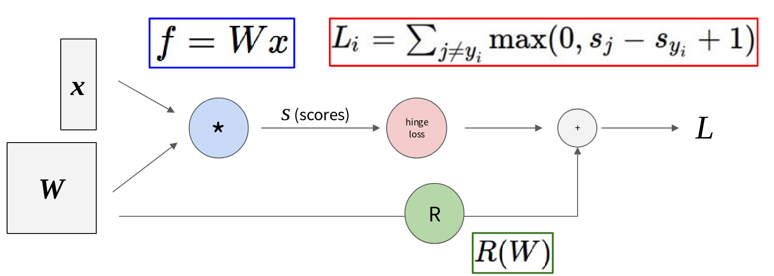
Let’s look at the example, which is for our familiar linear classifier with hinge loss and regularization.

1. We start with our inputs \(x\) and our weights \(W\).
2. The first operation is computing the scores: \(s = Wx\). This is represented by a node. It takes \(W\) and \(x\) as inputs and produces scores \(S\).
3. These scores \(S\) then feed into the hinge loss function \(L_i = \sum \max(0, s_j - s_{y_i} + 1)\). This is another node in our graph.
4. Separately, our weights \(W\) also feed into a regularization function \(R(W)\).
5. Finally, the output of the hinge loss (\(L_i\), which would then be averaged over the batch) and the output of the regularization term \(R(W)\) are added together (the + node) to give us our final total loss \(L\).

So, we’ve decomposed our complex loss calculation into a directed acyclic graph of basic operations. Each node in this graph takes some inputs and produces an output. The beauty of this approach is that if we know how to compute the local gradient for each elementary operation for example how does the output of the \(Wx\) node change if \(W\) changes a little?, we can then use the chain rule from calculus to systematically “backpropagate” the gradient of the final loss \(L\) all the way back to our input parameters \(W\). This “backpropagation” algorithm is the workhorse that allows us to efficiently compute gradients for arbitrarily complex neural networks. It’s modular because we only need to know the local derivative for each type of node (matrix multiply, addition, ReLU, sigmoid, loss function, etc.). And it’s systematic, meaning we can implement it once, and it will work for any network architecture we can express as a computational graph. This approach is essential for handling the complexity of modern deep learning models.

Think about Convolutional Network like AlexNet, which was a groundbreaking architecture for image recognition. Trying to write down the full analytical derivative of the loss with respect to all those different sets of weights in AlexNet would be an absolute nightmare. It’s just too complex. And it gets even crazier. Consider something like a Neural Turing Machine. This is a type of neural network architecture that’s augmented with an external memory component that it can learn to read from and write to. The idea is to give the network capabilities closer to a traditional computer program. The computational graph for a Neural Turing Machine, especially if you unroll its operations over time becomes incredibly deep and complex. Each “time step” of the machine’s operation adds another layer to this graph. Again, attempting to derive gradients by hand for such a system is completely out of the question. So, for all these sophisticated architectures – from convolutional networks to these very deep and recurrent models – we absolutely need a robust, general, and efficient method for computing gradients. And that method is backpropagation, operating on these computational graphs.

Backpropagation

So the solution backpropagation. This is the algorithm that will allow us to compute these gradients efficiently and systematically. It’s essentially a practical application of the chain rule from calculus on a computational graph. Let’s illustrate backpropagation with a simple example. Consider the function \(f(x, y, z) = (x + y) * z\). Our goal will be to compute the partial derivatives of \(f\) with respect to \(x\), \(y\), and \(z\), that is, \(\frac{\partial f}{\partial x}\), \(\frac{\partial f}{\partial y}\), and \(\frac{\partial f}{\partial z}\). First, let’s represent this function as a computational graph

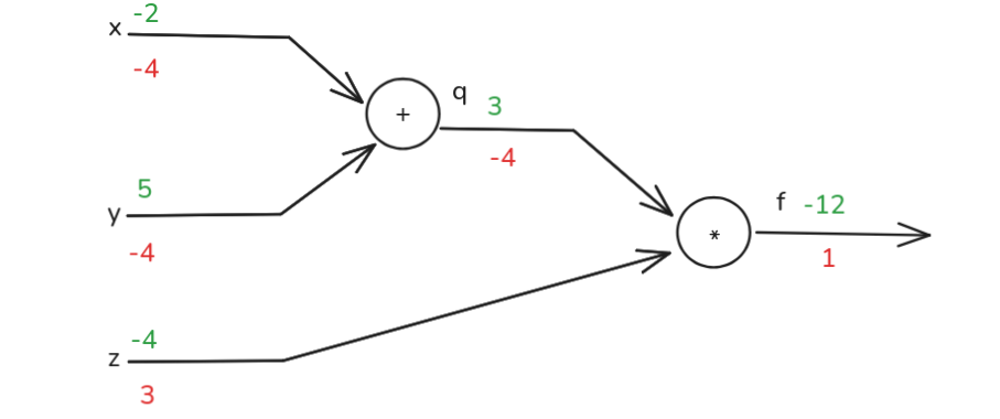
We have inputs \(x\) and \(y\). These are fed into an addition node. Let’s call the output of this addition \(q\). So, \(q = x + y\). Then, this intermediate value q and our third input \(z\) are fed into a multiplication node. The output of this multiplication node is our final function value \(f\). So, \(f = q z\). This graph breaks the computation down into two simple steps: an addition and a multiplication. Now, let’s assign some concrete values to our inputs to trace the computation. Let’s say, for example, \(x = -2\), \(y = 5\), and \(z = -4\), so \(q = 3\) and \(f = -12\). This is the forward pass: we compute the values of all nodes in the graph from inputs to output.

Now, for backpropagation, we need the local gradients for each node in our graph. That is, for each operation, we need to know how its output changes with respect to its inputs. Consider the first operation: \(q = x + y\), \(\frac{\partial q}{\partial x} = 1\) so if \(x\) changes by a small amount, \(q\) changes by that same amount, similarly \(\frac{\partial q}{\partial y} = 1\). These are the local gradients for the addition gate. Next, consider the second operation: \(f = q z\). \(\frac{\partial f}{\partial q} = z\) so if \(q\) changes by a small amount \(dq\), \(f\) changes by \(z \cdot dq\). And \(\frac{\partial f}{\partial z} = q\), if z changes by a small amount \(dz\), \(f\) changes by \(q \cdot dz\). So, we have the local derivatives for each individual operation. Ultimately, what we want are the gradients of the final output \(f\) with respect to the initial inputs \(x\), \(y\), and \(z\): \(\frac{\partial f}{\partial x}\), \(\frac{\partial f}{\partial y}\) and \(\frac{\partial f}{\partial z}\).

Okay, we’re ready to start the backward pass. We work from the output \(f\) back towards the inputs \(x, y, z\). The very first gradient we consider is the gradient of the final output \(f\) with respect to itself, \(\frac{\partial f}{\partial f}\). This is always 1, by definition. This ‘1’ is often called the initial “upstream gradient”, it’s the gradient that starts the whole backward flow. You can see it annotated on the graph in read next to \(f\).

Now let’s move back one step, we want to find \(\frac{\partial f}{\partial z}\). \(z\) is an input to the multiplication gate \(f = qz\) The local gradient of \(f\) with respect to \(z\) is \(q\). From our forward pass, we know \(q = 3\). So, \(\frac{\partial f}{\partial z} = 3\). The upstream gradient \(\frac{\partial f}{\partial f}\) (which is 1) is multiplied by the local gradient \(\frac{\partial f}{\partial z}\) (which is q). So, \(1 q = q = 3\). This value 3 is now the gradient of the final output \(f\) with respect to the node \(z\).

Next, we want \(\frac{\partial f}{\partial q}\). \(q\) is the other input to the multiplication gate \(f = qz\). The local gradient of \(f\) with respect to \(q\) is \(z\). From our forward pass, \(z = -4\). So, \(\frac{\partial f}{\partial q} = -4\). Again the upstream gradient \(\frac{\partial f}{\partial f}\) (which is 1) multiplied by the local gradient \(\frac{\partial f}{\partial q}\) (which is z). So, \(1 \cdot z = z = -4\). This \(-4\) is the gradient of the final output \(f\) with respect to the intermediate node \(q\). This value will be crucial as we continue propagating backward, because \(q\) itself depends on \(x\) and \(y\).

Now we need to go further back to get \(\frac{\partial f}{\partial y}\). \(y\) is an input to the addition gate \(q = x + y\). The node \(y\) influences \(f\) through \(q\). This is where the chain rule comes into play. The chain rule tells us:

\[ \frac{\partial f}{\partial y}= \frac{\partial f}{\partial q} \frac{\partial q}{\partial y} \]

\(\frac{\partial f}{\partial q}\) is the gradient of the final output \(f\) with respect to \(q\). We just calculated this as \(-4\). This is often called the upstream gradient coming into the \(q\) node from later parts of the graph. \(\frac{\partial q}{\partial y}\) is the local gradient of the \(q\) node with respect to its input \(y\). From \(q = x + y\), we know \(\frac{\partial q}{\partial y} = 1\). So, \(\frac{\partial f}{\partial y} = -4 \cdot 1 = -4\). This \(-4\) is now the gradient of the final output \(f\) with respect to the input \(y\).

Finally, let’s get \(\frac{\partial f}{\partial x}\) Similar to \(y, x\) is an input to the addition gate \(q = x + y\), and it influences \(f\) through \(q\), we apply the chain rule here \(\frac{\partial f}{\partial x} = \frac{\partial f}{\partial q} \frac{\partial q}{\partial x}\). So, \(\frac{\partial f}{\partial x} = -4 \cdot 1 = -4\). This \(-4\) is the gradient of the final output \(f\) with respect to the input \(x\).

So, to summarize, we’ve found:

\[ \begin{align} \frac{\partial f}{\partial f} &= 1 \\ \frac{\partial f}{\partial z} &= q = 3 \\ \frac{\partial f}{\partial q} &= z = -4 \\ \frac{\partial f}{\partial y} &= \frac{\partial f}{\partial q} \frac{\partial q}{\partial y} = -4 \cdot 1 = -4 \\ \frac{\partial f}{\partial x} &= \frac{\partial f}{\partial q} \frac{\partial q}{\partial x} = -4 \cdot 1 = -4 \end{align} \]

Let’s generalize this idea of backpropagation through a single computational gate.

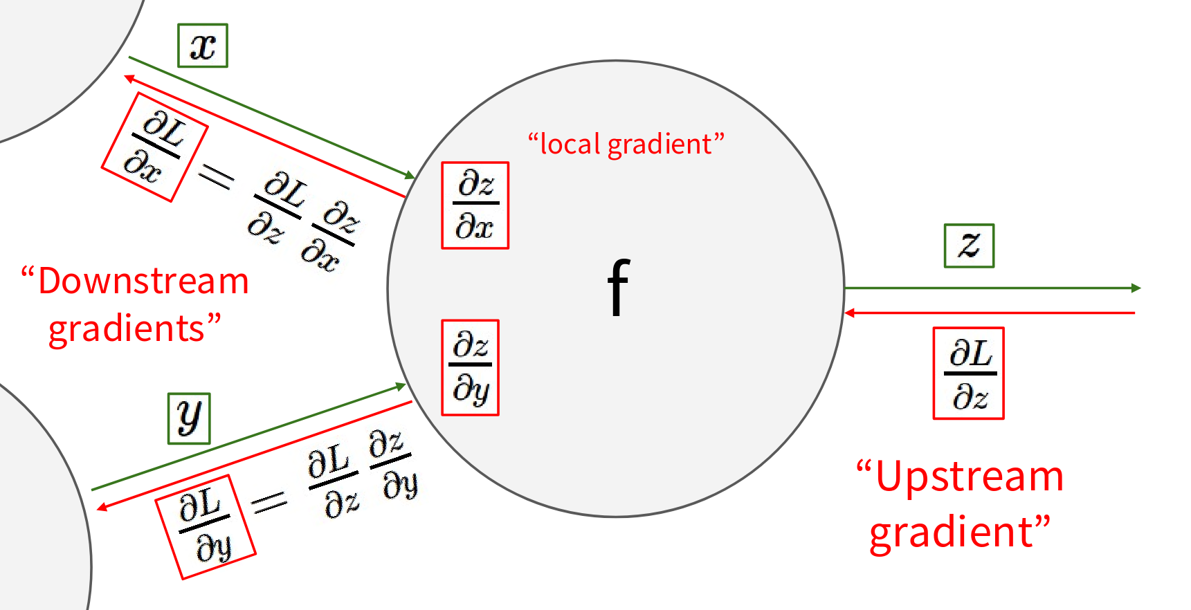
Imagine we have some generic function, or “gate,” \(f\). This gate takes some inputs, let’s say \(x\) and \(y\), and it produces an output \(z\). This \(f\) could be an addition, a multiplication, a ReLU, a sigmoid, any elementary operation. For this gate to be part of a backpropagation process, we need to know its local gradients. These are the partial derivatives of the gate’s output \(z\) with respect to each of its inputs, \(x\) and \(y\) So, we need to be able to compute \(\frac{\partial z}{\partial x}\) and \(\frac{\partial z}{\partial y}\) . These gradients tell us how a small change in x (or y) directly affects z, assuming all other inputs to this specific gate are held constant. Now, during the backward pass, this gate \(f\) will receive an upstream gradient. This upstream gradient is the derivative of the final loss function \(L\) which is at the very end of our entire computational graph with respect to the output of this gate, \(z\). So, we receive \(\frac{\partial L}{\partial z}\). This \(\frac{\partial L}{\partial z}\) tells us how much the final loss \(L\) changes if the output \(z\) of this particular gate changes by a small amount. This gradient has been propagated backward from later parts of the graph. Our goal, when backpropagating through this gate, is to compute the Downstream gradients. These are the derivatives of the final loss \(L\) with respect to the inputs of this gate, \(x\) and \(y\). So, we want to calculate \(\frac{\partial L}{\partial x}\) and \(\frac{\partial L}{\partial y}\). How do we do this? We use the chain rule. To find \(\frac{\partial L}{\partial x}\), we multiply the upstream gradient \(\frac{\partial L}{\partial z}\) by the local gradient \(\frac{\partial z}{\partial x}\):

\[ \frac{\partial L}{\partial x}= \frac{\partial L}{\partial z} * \frac{\partial z}{\partial x} \]

This tells us how much the final loss \(L\) changes if the input \(x\) to this gate changes by a small amount. And similarly for the input \(y\). So, for any gate in our computational graph, if we know its local gradient and the upstream gradient coming into its output we can compute the downstream gradient which will then become the upstream gradients for the gate that produced \(x\) and \(y\). This process is then repeated for every gate in the graph, working backwards from the final loss. Each gate receives an upstream gradient from its successor(s) in the forward pass. It uses this, along with its own local gradients, to compute downstream gradients. These downstream gradients are then passed further back to its predecessor(s). This recursive application of the chain rule is what allows us to efficiently compute the gradient of the overall loss function with respect to all parameters and inputs in the network. This pattern of upstream gradient times local gradient gives downstream gradient is the fundamental computation performed at each node during backpropagation.

Okay, let’s look at another example This time, the function is

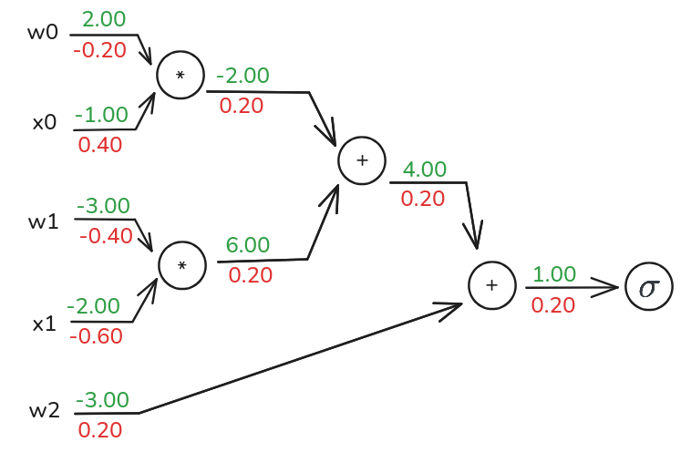
\[ f(w, x) = \frac{1}{1 + e^{-(w_0x_0 + w_1x_1 + w_2)}} \]

This should look familiar! It’s the sigmoid function applied to a linear combination of inputs \(w_0x_0 + w_1x_1 + w_2\). This is exactly what one neuron in a neural network might compute if it’s using a sigmoid activation. Our goal will be to find the gradients of this f with respect to \(w_0, x_0, w_1, x_1\), and \(w_2\). And if we work it out like the previous example we would have this graph

Sigmoid function: \(\sigma(x) = \frac{1}{1 + e^{-x}}\)

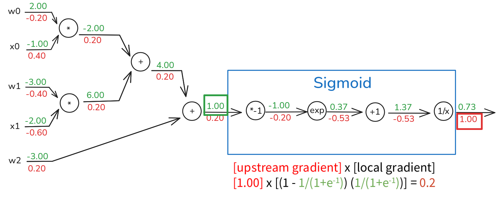
Now, let’s take a step back and look at a section of this graph. The sequence of operations we performed multiply by -1 then exp then add 1, then take reciprocal (1/x) – this entire chain, highlighted in the blue box, is actually the computation of the Sigmoid function. The input to this entire sigmoid block was the value 1.00 and the output of the sigmoid block was 0.73. An important point here is that the computational graph representation may not be unique. We can choose to break down functions into very fine-grained elementary operations, as we did, or we can group common sequences of operations into a single “macro” gate. The key is to choose a representation where the local gradients at each node can be easily expressed. So, instead of backpropagating through each of those four individual steps, we could have treated the entire sigmoid function as a single gate. To do that, we’d need the sigmoid local gradient. The derivative of the sigmoid function with respect to its input \(x\) is a well-known result:

\[ \frac{d \sigma(x)}{d x} = \frac{e^{-x}}{\left(1 + e^{-x}\right)^2} = \left( \frac{1 + e^{-x} - 1}{1 + e^{-x}}\right) \left(\frac{1}{1 + e^{-x}}\right) = \left(1 - \sigma(x)\right) \sigma(x) \]

This is a very convenient form because it expresses the derivative in terms of the function’s own output value. So, if we treat the sigmoid as a single gate. The input to this sigmoid gate was \(x\_in = 1.00\). The output was \(\sigma(x\_in) = 0.73\). The upstream gradient coming into the output of the sigmoid gate was 1.00. The local gradient of the sigmoid function, evaluated at its input \(x\_in=1.00\), is \(\sigma(1.00) (1 - \sigma(1.00))\). Since \(\sigma(1.00)\) is approximately \(0.73\), the local gradient is \(0.73 \cdot (1 - 0.73) = 0.73 \cdot 0.27 \approx 0.1971\). Then we calculate the downstream gradient which is \(upstream\_gradient \cdot (1-\sigma(1)) \sigma(1)\) and this evaluates to approximately 0.2. And if you look back at our step-by-step backpropagation, the gradient we computed at the input of the multiply by -1 gate which was the start of our sigmoid block was indeed 0.20! This demonstrates the modularity of backpropagation. We can define common operations like sigmoid, ReLU, tanh, etc., as single “black-box” gates. As long as we know how to compute their output during the forward pass and their local gradient during the backward pass, we can easily plug them into any computational graph. Modern deep learning frameworks are built around this idea of a library of predefined layers or operations, each knowing its forward and backward computation. This ability to abstract away complex operations into single gates with well-defined local gradients is incredibly powerful and makes implementing backpropagation for complex architectures much more manageable.

Backpropagation in practice

Now, let’s look for some general patterns in how these gradients flow through different types of gates. Understanding these can give you a good intuition for how backpropagation works.

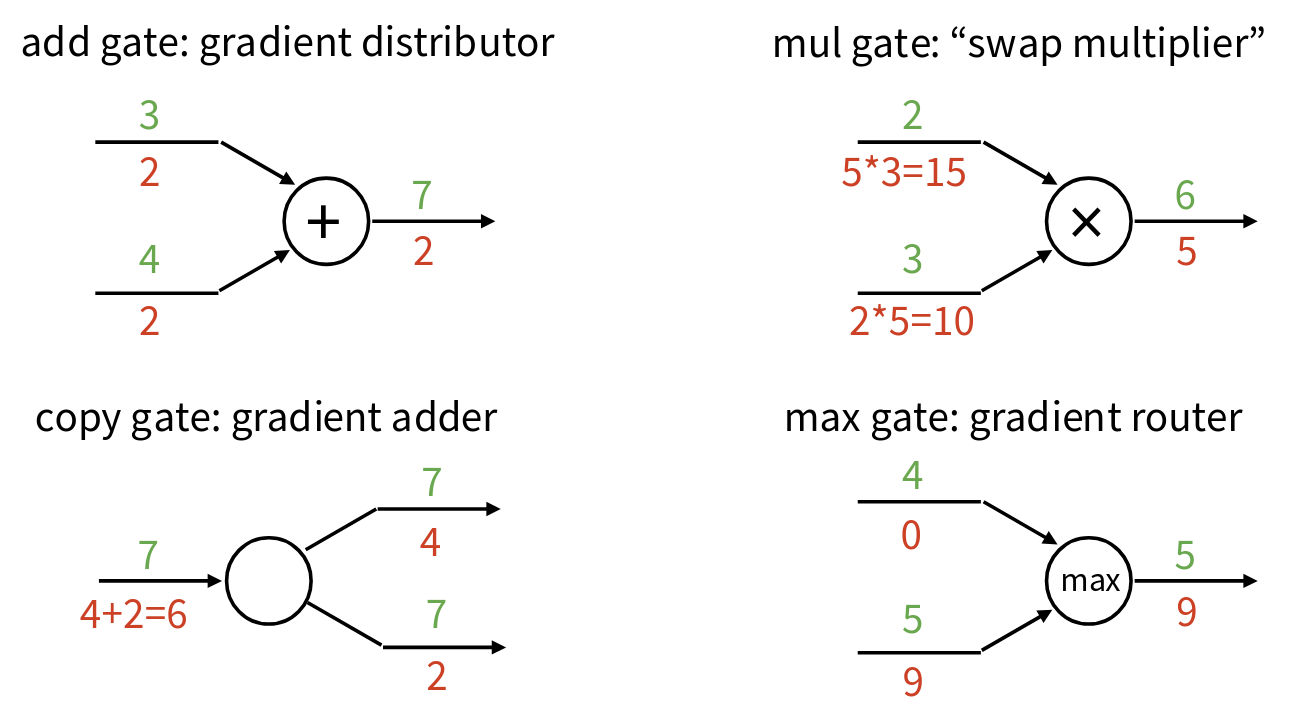
First, let’s consider the add gate: \(z = x + y\). The add gate acts as a gradient distributor. It takes the upstream gradient and simply passes it along (distributes it) to both of its inputs unchanged, because the local gradients are 1.

Next, the mul gate (multiplication gate): \(z = x y\). The mul gate acts as a swap multiplier. The gradient \(\frac{dL}{dx}\) is the upstream gradient times the other input \(y\). And \(\frac{dL}{dy}\) is the upstream gradient times the other input \(x\). It’s like the inputs get swapped when they multiply the upstream gradient.

What about a copy gate? A copy gate is when a single input \(x\) is used in multiple places further down the graph. During backpropagation, this means gradients from multiple paths will flow back to x. A copy gate (or a “fan-out” point) acts as a gradient adder. It sums up all the incoming upstream gradients. This is a direct consequence of the multivariate chain rule when a variable influences the loss through multiple paths.

Finally, consider a max gate: \(z = \max(x, y)\). The max gate acts as a gradient router. It takes the upstream gradient and routes it entirely to the input that won (had the maximum value) during the forward pass. The gradient for the input that lost is zero. This makes sense if \(x\) wasn’t the max, then small changes in x (as long as it stays not the max) won’t affect the output \(z\) at all.

These patterns of distributor for add, swap multiplier for mul, adder for copy, and router for max are very useful to keep in mind when thinking about how gradients propagate through a network. ReLU, for example, \(\max(0, x)\), is a special case of the max gate. If \(x > 0\), the gradient passes through. If \(x <= 0\), the gradient becomes zero.

So, we have this conceptual understanding of backpropagation using computational graphs. How do we actually implement this? One way is to write “Flat” code. This means we explicitly write out the sequence of operations for the forward pass and then, in reverse order, write out the corresponding operations for the backward pass. Let’s look at our sigmoid example again

def f(w0, x0, w1, x1, w2):
  s0 = w0 * x0  # Forward pass
  s1 = w1 * x1
  s2 = s0 + s1
  s3 = s2 + w2
  L = sigmoid(s3)


  grad_L = 1.0 # Backward pass
  grad_s3 = grad_L * (1 - L) * L
  grad_w2 = grad_s3
  grad_s2 = grad_s3
  grad_s0 = grad_s2
  grad_s1 = grad_s2
  grad_w1 = grad_s1 * x1
  grad_x1 = grad_s1 * w1
  grad_w0 = grad_s0 * x0
  grad_x0 = grad_s0 * w0

During this forward pass, we would typically store all the intermediate values s0, s1, s2, s3 and the final output L, because we’ll need them for the backward pass. Now, for the Backward pass to compute the gradients we work backward from the last operation in the forward pass. And that’s it! We’ve computed all the gradients we needed. Notice how the backward pass code mirrors the forward pass code but in reverse order. Each line in the forward pass that computes some variable v will have a corresponding set of lines in the backward pass that compute grad_v (the gradient of the final loss with respect to v) and then use grad_v to compute gradients for the inputs to that operation. This “flat” style of implementation is straightforward for simple functions. However, for very deep or complex networks, writing out all these steps explicitly can become tedious and error-prone. We’d prefer a more modular approach.

A much better approach for practical deep learning systems is a modularized implementation using a well-defined forward / backward API for each type of gate or operation. The idea is that each elementary operation (like multiplication, addition, sigmoid, ReLU, convolution, etc.) is implemented as an object or a set of functions that knows two things: 1) how to compute its output given its inputs (the forward pass). 2) how to compute the gradients with respect to its inputs, given the gradient with respect to its output (the backward pass). Here’s an example of what this might look like, using syntax similar to what you’d find in PyTorch’s autograd.Function.

class Multiply(torch.autograd.Function):
  @staticmethod
  def forward(ctx, x, y):
1    ctx.save_for_backward(x, y)
    z = x * y
    return z

  @staticmethod
2  def backward(ctx, grad_z):
    x, y = ctx.saved_tensors
    grad_x = y * grad_z
    grad_y = x * grad_z
    return grad_x, grad_y

1

We need to cache some values for use in backward

2

grad_z is upstream gradient

This is the pattern. Every operation (or “layer” in a deep learning framework) will have a forward method that computes its output and stashes away anything needed for the backward pass, and a backward method that takes the upstream gradient and uses the stashed values and local derivatives to compute and return the downstream gradients.

Backpropagation with vectors and matrices

So far, we’ve mostly been talking about scalar inputs and outputs for these gates. But in neural networks, we usually deal with vectors, matrices and tensors. All the examples we’ve worked through like \(f(x,y,z) = (x+y)z\) and the sigmoid example \(f(w,x) = \sigma(w_0x_0 + w_1x_1 + w_2)\) involved scalar inputs and scalar intermediate values. But in real neural networks, our inputs x are often vectors (e.g., an image flattened into a vector), our weights W are matrices, and the outputs of layers are vectors or higher-dimensional tensors. So, the question is what about vector-valued functions? How does backpropagation work then? To answer this, let’s quickly recap vector derivatives.

Scalar to Scalar, if we have a scalar input \(x \in \mathbb{R}\) and a scalar \(y \in \mathbb{R}\), then we have the regular derivative \(\frac{dy}{dx}\). This tells us: if x changes by a small amount, how much will y change? The derivative itself is also a scalar \(\frac{dy}{dx} \in \mathbb{R}\).

Vector to Scalar, now what if our input \(x \in \mathbb{R}^N\) (a vector) and \(y \in \mathbb{R}\) (a scalar). The derivative is now the Gradient \(\frac{\partial y}{\partial x} \in \mathbb{R}\) where n-th component is \(\left(\frac{\partial y}{\partial x}\right)_n = \frac{\partial y}{\partial x_n}\). This gradient answers the question for each element of \(x\), if it changes by a small amount, then how much will \(y\) change? Our loss function \(L\) is a scalar, and our weights \(W\) (and inputs x to various layers) are often vectors or matrices. So, when we compute \(\frac{\partial L}{\partial W}\), we are computing a gradient.

Vector to Vector, what if both our input \(x \in \mathbb{R}^N\) (a vector) and our output \(y \in \mathbb{R}^M\) (a vector). The derivative is now the Jacobian matrix \(\frac{\partial y}{\partial x} \in \mathbb{R}^{N \times M}\). This is an \(M \times N\) matrix, where the element at row \(m\), column \(n\) is \(\left(\frac{\partial y}{\partial x}\right)_{n,m} = \frac{\partial y_m}{\partial x_n}\). This Jacobian answers the question for each element of \(x\), if it changes by a small amount, then how much will each element of y change? Many layers in a neural network can be thought of as vector-to-vector functions (e.g., a fully connected layer maps an input vector to an output vector of activations). The chain rule still applies, but now it involves matrix-vector multiplications or Jacobian-vector products. Let’s see how this plays out.

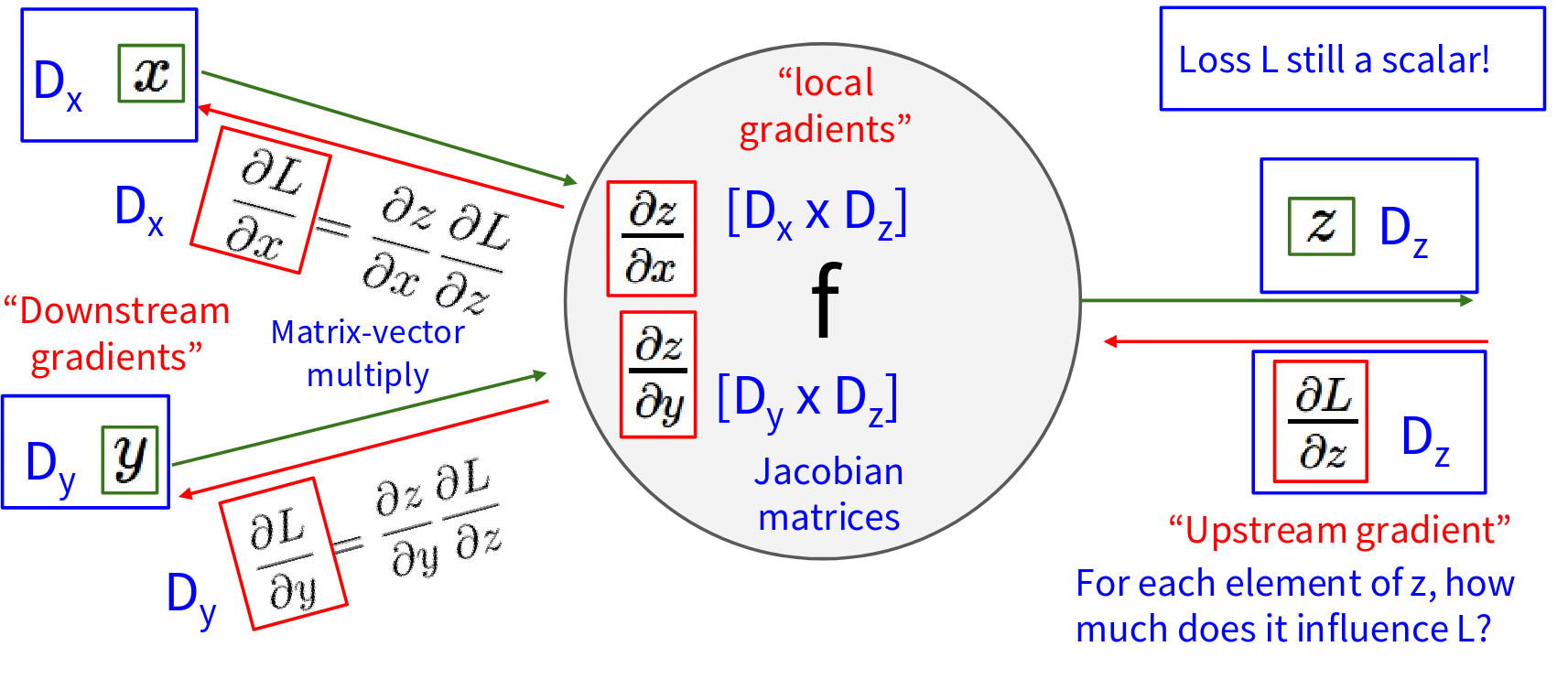
We still have our gate \(f\) which takes inputs, say \(x\) and \(y\), and produces an output \(z.\) Crucially, the final Loss \(L\) is still a scalar! We are always trying to minimize a single scalar value representing how bad our network’s predictions are. During the backward pass, this gate will receive an Upstream gradient. This is the gradient of the scalar Loss L with respect to the vector output z of this gate. So, it’s \(\frac{\partial L}{\partial z}\). Since \(L\) is a scalar and \(z\) is a D_z-dimensional vector, this upstream gradient \(\frac{\partial L}{\partial z}\) will also be a D_z-dimensional vector. It tells us: “For each element of \(z\), how much does that element influence the final Loss \(L\)?”. Now, the “local gradients” for this gate \(f\) describe how its output z changes with respect to its inputs \(x\) and \(y\). \(\frac{\partial z}{\partial x}\): Since \(z\) is D_z-dim and \(x\) is D_x-dim, this is the Jacobian matrix of \(z\) with respect to \(x\) and same with \(y\). The shapes of these Jacobians:

• \(\frac{\partial z}{\partial x}\) will be a D_x x D_z matrix (derivative of each component of \(z\) w.r.t. each component of \(x\)).
• \(\frac{\partial z}{\partial y}\) will be a D_y x D_z matrix.

The Downstream gradients we want to compute are \(\frac{\partial L}{\partial x}\) (a D_x-dim vector) and \(\frac{\partial L}{\partial y}\) (a D_y-dim vector). Using the chain rule:

\[ \begin{align} \frac{\partial L}{\partial x} &= \frac{\partial z}{\partial x} \frac{\partial L}{\partial z} \\ \frac{\partial L}{\partial y} &= \frac{\partial z}{\partial y} \frac{\partial L}{\partial z} \end{align} \]

An important principle to remember: Gradients of variables with respect to the loss have the same dimensions as the original variable.

• \(x\) is a D_x-dimensional vector. Its gradient \(\frac{\partial L}{\partial x}\) is also a D_x-dimensional vector.
• \(y\) is a D_y-dimensional vector. Its gradient \(\frac{\partial L}{\partial y}\) is also a D_y-dimensional vector.
• \(z\) is a D_z-dimensional vector. Its upstream gradient \(\frac{\partial L}{\partial z}\) is also a D_z-dimensional vector

This makes intuitive sense: for every element in a variable (like a weight matrix or an activation vector), we need a corresponding gradient value that tells us how changing that specific element affects the final scalar loss. This consistency of shapes is critical for implementing backpropagation correctly in code

Let’s walk through a concrete example of backprop with vectors, using an element-wise ReLU function, \(f(x) = \max(0,x)\)

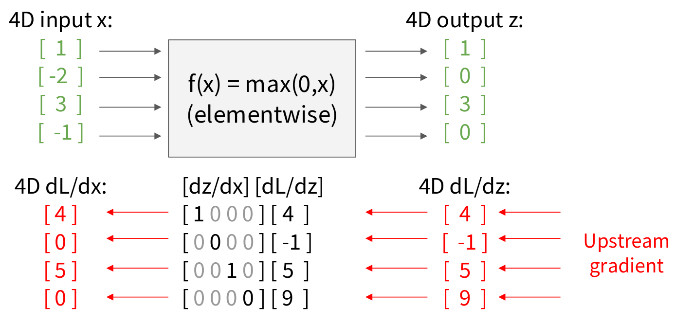
We have a 4D input vector x as shown in the image, and the function max(0,x) is applied element-wise, and the output vector z. Now, for the backward pass, let’s assume we’ve received the upstream gradient \(\frac{\partial L}{\partial z}\) This \(\frac{\partial L}{\partial z}\) is also a 4D vector. Let’s say it’s \(\left[4, -1, 5, 9\right]^T\). This tells us, for example, that if the first element of \(z\) changes by a small amount, the loss \(L\) changes by 4 times that amount. To compute the downstream gradient \(\frac{\partial L}{\partial x}\), we need the Jacobian matrix \(\frac{\partial z}{\partial x}\). Since \(z_i = \max(0, x_i)\), the output \(z_i\) only depends on the corresponding input \(x_i\). It does not depend on \(x_j\) for \(j \neq i\). This means the Jacobian matrix will be diagonal.

• If \(x_i > 0\), then \(z_i = x_i\), so \(\frac{\partial z_i}{\partial x_i} = 1\).
• If \(x_i \leq 0\), then \(z_i = 0\), so \(\frac{\partial z_i}{\partial x_i} = 0\).

So, the Jacobian \(\frac{\partial z}{\partial x}\) is a 4x4 diagonal matrix. Now, we compute \(\frac{\partial L}{\partial x}\) = \(\frac{\partial z}{\partial x}\) \(\frac{\partial L}{\partial z}\). This is a matrix-vector multiplication

Notice something important here. For element-wise operations like ReLU, the Jacobian is sparse, and specifically, it’s diagonal. The off-diagonal entries are always zero. Because of this, we Never explicitly form the full Jacobian matrix in practice for these types of operations. That would be very inefficient, especially for high-dimensional vectors. Storing a large D x D diagonal matrix is wasteful if only D elements are non-zero. Instead, we use implicit multiplication. We know that multiplying by a diagonal matrix is equivalent to an element-wise product with the diagonal elements

\[ \left(\frac{\partial L}{\partial x}\right)_i = \begin{cases} \left(\frac{\partial L}{\partial z}\right)_i & \text{ if } x_i > 0 \\ 0 & \text{otherwise} \end{cases} \]

This is far more efficient than forming the full Jacobian and doing a matrix-vector multiply. Most deep learning frameworks will implement backpropagation through element-wise operations like this, using element-wise masking or multiplication. So, while the concept of Jacobians is important for understanding the general case, for many common operations, we can exploit their structure to make the backward pass much more efficient.

Now, what about when our variables are not just vectors, but matrices or even higher-dimensional tensors? So let’s extend this to backprop with matrices (or tensors). The good news is that the core principles remain exactly the same. We still have our gate f, Our inputs x and y can now be matrices (or higher-order tensors). Let’s say x is D_x x M_x and y is D_y x M_y. The output z is also a matrix, say D_z x M_z. The Loss L is still a scalar! This is always true. And remember, \(\frac{\partial L}{\partial x}\) will always have the same shape as x. So \(\frac{\partial L}{\partial x}\) will be a D_x x M_x matrix of gradients.

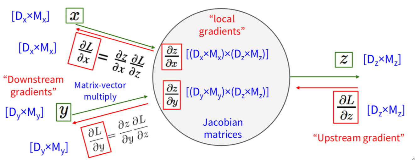
The local gradients are still conceptually Jacobian matrices, but now they relate elements of input matrices to elements of the output matrix. The chain rule, downstream = local * upstream, still holds. However, explicitly forming these Jacobians when \(x\), \(y\), and \(z\) are matrices would involve thinking about derivatives of matrices with respect to matrices, which can lead to 4th-order tensors and becomes very cumbersome to write down and implement directly. Instead, what usually happens in practice is that we consider the matrix operations themselves (like matrix multiplication, element-wise operations on matrices, etc.) and derive the gradient expressions for those specific operations directly, often by thinking about how a small change in an input matrix element affects an element in the output matrix, and then summing up contributions to the scalar loss. The result is usually an expression for the gradient matrix \(\frac{\partial L}{\partial X}\) that has the same shape as \(X\) and can be computed efficiently. The dimensions of these abstract Jacobians would be:

• \(\frac{\partial z}{\partial x}\) relating a (D_x x M_x) input to a (D_z x M_z) output.
• \(\frac{\partial z}{\partial y}\) relating a (D_y x M_y) input to a (D_z x M_z) output.

These would be very high-dimensional objects if we thought of them explicitly. The key takeaway is that even though the underlying math involves Jacobians of matrix-valued functions, for common operations like matrix multiplication, element-wise functions, convolutions, etc., we have pre-derived, efficient formulas for computing the gradient \(\frac{\partial L}{\partial X}\) given \(\frac{\partial L}{\partial Z}\) and the original inputs, and these formulas maintain the correct shapes.

Let’s look at a very common example: matrix multiplication.

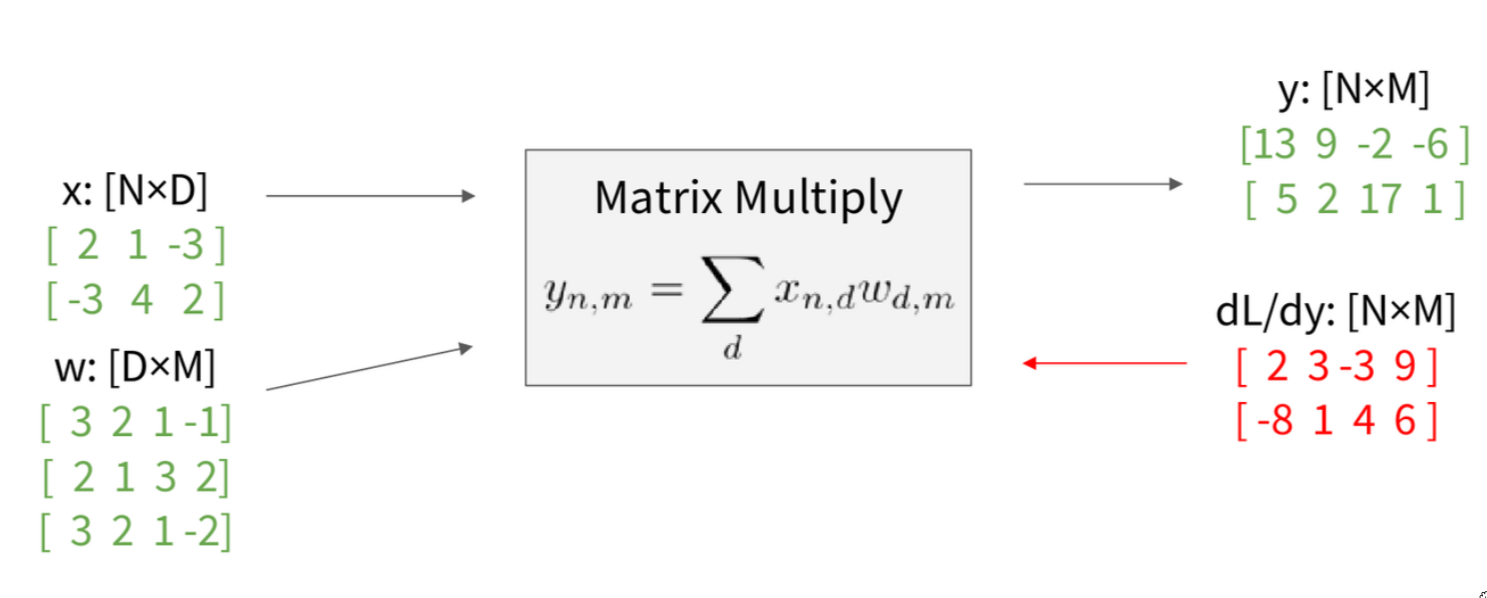
We have an input matrix \(x\) of size N x D, and a weight matrix \(w\) of size D x M. The output \(y\) is their product: \(y = x w\). This output \(y\) will be an N x M matrix. The formula for an element \(y_{n,m}\) of the output is \(y_{n,m} = \sum_d (x_{n,d} w_{d,m})\). This is the standard definition of matrix multiplication – the dot product of the n-th row of \(x\) with the m-th column of \(w.\) We are given the upstream gradient \(\frac{\partial L}{\partial y}\), which is an N x M matrix, having the same shape as \(y\). Our goal is to find \(\frac{\partial L}{\partial x}\) (an N x D matrix) and \(\frac{\partial L}{\partial w}\) (a D x M matrix). Now, if we were to think about the Jacobians explicitly, the Jacobian \(\frac{\partial y}{\partial x}\) would relate an (N x D) input to an (N x M) output, the Jacobian \(\frac{\partial y}{\partial z}\) would relate a (D x M) input to an (N x M) output. These would be 4D tensors! For example, if N=64 (batch size), D=M=4096 (common hidden layer sizes), then NxD is roughly 250,000, and NxM is also roughly 250,000. So the Jacobian \(\frac{\partial y}{\partial x}\) would have (ND) (N*M) elements, which is about (2.5e5)^2 = 6.25e10 elements. If each is a 4-byte float, that’s 250 GB of memory just for one Jacobian! Clearly, we must work with them implicitly! We cannot afford to form these giant Jacobian tensors. So, let’s reason about it element by element. What parts of \(y\) are affected by one element of \(x\)? Let’s consider \(x_{n,d}\). The element \(x_{n,d}\) affects the whole n-th row of y (e.g., \(y_{n,:}\)), this is because \(x_{n,d}\) participates in the calculation of \(y_{n,m}\) for all values of \(m\). So, to find \(\frac{\partial y}{\partial x_{n,d}}\), we need to sum up the influence of \(x_{n,d}\) on each \(y_{n,m}\) and then how each \(y_{n,m}\) influences \(L\). Using the chain rule:

\[ \frac{\partial y}{\partial x_{n,d}} = \sum_m{ \frac{\partial L}{\partial y_{n,m}} \frac{\partial y_{n,m}}{\partial x_{n,d}}} \]

Now, let’s look at the local derivative \(\frac{\partial y_{n,m}}{\partial x_{n,d}}\). From \(y_{n,m} = \sum_k{ x_{n,k} w_{k,m}}\), if we vary \(x_{n,d}\), how does \(y_{n,m}\) change? Well, \(x_{n,d}\) is multiplied by \(w_{d,m}\) to contribute to \(y_{n,m}\). So

\[ \begin{align} \frac{\partial y_{n,m}}{\partial x_{n,d}} &= w_{d,m} \\ \frac{\partial L}{\partial x_{n,d}} &= \sum_m \frac{\partial L}{\partial y_{n,m}} w_{d,m} \end{align} \]

And that sum is exactly the formula for the (n,d)-th element of the matrix product \(\frac{\partial L}{\partial y} w^T\). So, in matrix form:

\[ \frac{\partial L}{\partial x} = \frac{\partial L}{\partial y} * w^T \]

Let’s check shapes

\[ \overbrace{\frac{\partial L}{\partial x}}^{N \times D} = \underbrace{\frac{\partial L}{\partial y}}_{N\times M}\; \overbrace{w^{\!T}}^{M\times D} \]

By similar logic for \(\frac{\partial L}{\partial w}\) , we can derive:

\[ \overbrace{\frac{\partial L}{\partial w}}^{ D \times M } = \underbrace{x^T}_{D \times N} \overbrace{\frac{\partial L}{\partial y}}^{N \times M} \]

And there’s a nice mnemonic: they are the only way to make the shapes match up! If you remember the input and output shapes, and that you need to use \(\frac{\partial L}{\partial y}\) and the other input matrix (or its transpose), you can often re-derive these just by making the dimensions work out for matrix multiplication. So, for a matrix multiply gate, given the upstream gradient \(\frac{\partial L}{\partial y}\) , we can directly compute the downstream gradients \(\frac{\partial L}{\partial x}\) and \(\frac{\partial L}{\partial w}\) using these matrix multiplication formulas, without ever forming the explicit giant Jacobian. This is how it’s done in practice.