Image classification is truly a core task in computer vision. It’s the simplest and most fundamental problem, and mastering it forms the basis for more complex tasks like object detection and segmentation.
What makes a cat a cat?
Let’s explicitly define image classification. The task is: given an input image, assign it one label from a predefine set of possible categories. If we have an image of a cat. Our system would label ‘cat’. Crucially for this task, we assume we are given a set of possible labels, like {dog, cat, truck, plane, …}. The model job is to pick the most appropriate label from this list for any given input image. We’re not asking it for generate new label or descriptions, just to categorize.
Now, this simple task of image to label hides a fundamental challenge in computer vision, what we call Semantic Gap. With an image what you see is a beautiful, tabby cat maybe with green eyes, you immediately understand it’s a living creature a pet, specifically a cat. But what the computer sees is a grid of numbers. The semantic gap is precisely this challenge: how do we bridge the enormous gap between these raw numerical pixel values (what computer sees) and the high-level semantic concepts that we human effortlessly understand? That’s the core problem we’re trying to solve in image classification, and indeed, in much of computer vision.
Now let’s look at why this is so hard for a computers. The world is messy, and images with a lot of variability.
One of the primitive challenge is Viewpoint variation. Take our friendly cat again. You see if from one angle. But what if the camera moved slightly? Or what if you’re looking at a different photo of a same cat from a completely different side, or from above, blow? The camera illustrated around the cat show different potential viewpoints. From these different angles, even if it’s the exact same physical cat, the resulting image (the grid of pixel values) will be drastically different. For us it’s still ‘a cat’. For a computer it’s a completely new set of numbers. Our model need to learn that all these wildly different arrangements of pixels still correspond to the same underlying object. This invariance viewpoints is a huge challenge.
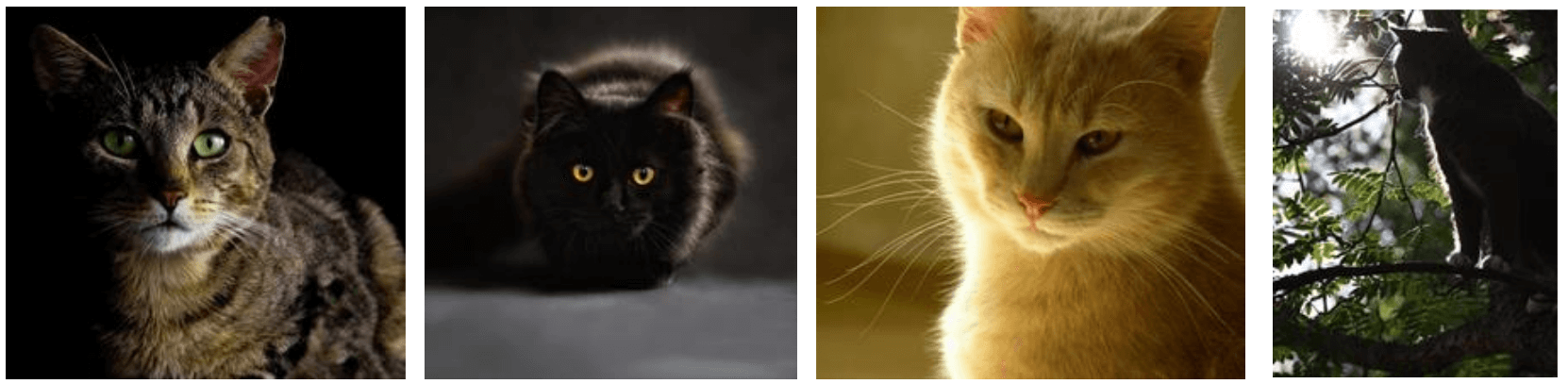
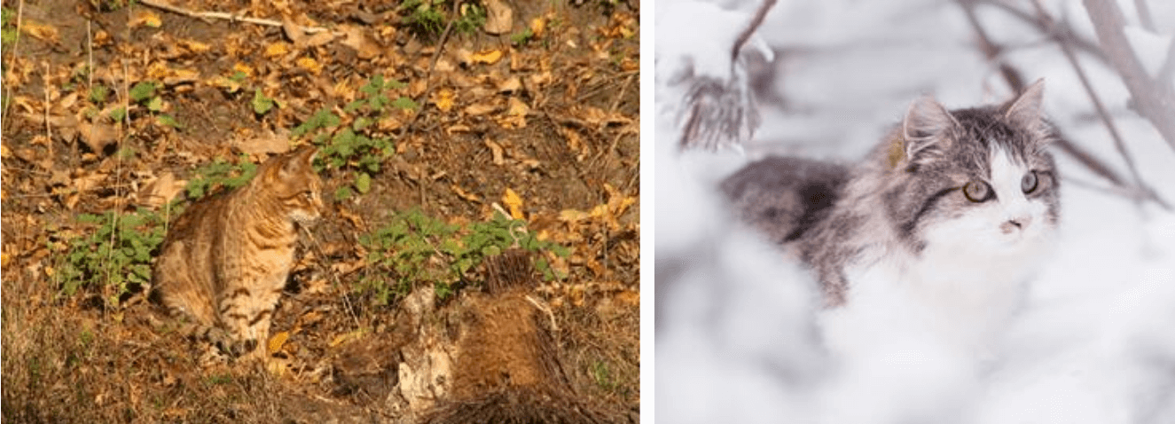
Another major hurdle is Illumination. The way an object is lit dramatically changes its appearance in an image. All of these are cat, but the pixel values, the color, the contrast they are completely different across these images due to varying light conditions. Our model must be robust enough to recognize a cat regardless of whether it’s in bright sunlight, deep snow, or under artifact light.
Then we have Background Clutter. Objects in real world rarely appears against a plain, uniform background. They are embedded in complex often messy environments. The challenge here is for the computer to distinguish the object of interest from everything else in the image. It needs to focus on the relevant features and ignore the distractors, even when the background is cluttered or has similar textures of colors.

A very common and difficult challenge is Occlusion. This occurs when parts of the object you’re trying to recognize are hidden from view from other objects. Despite missing large portion of the object, as human, we can still easily identify the cat. For a computer, dealing with these partial view and reasoning about what’s missing is incredibly difficult. It needs to learn to recognize an object even when only some of its characteristic features are present, or when they are distorted by being partially covered.
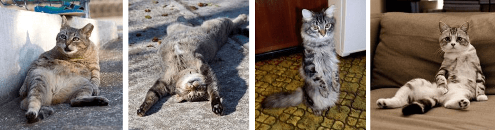
Another significant challenge is deformation. Many objects especially animate ones like animals and people, are not rigid They can change their shape, their pose, their configuration in countless ways. These are all cats, but their body shapes and the relative position of their limbs are drastically different. This isn’t just about camera moving around a rigid object, the object itself is deforming. Our visual system needs to be able to recognize an object class despite these non-rigid transformation. A simple template or a fix set of geometric rule would struggle immensely with these level of variability.
And if deformation wasn’t enough, we also have the huge challenge of Intraclass variation. What this means is that even within a single category, like ‘cat’ there can be an enormous amount of visual diversity. Think about different breed of cats look very different, they come in all sorts of colors and patterns. A good image classifier need to learn a concept of ‘cat’ that is general enough that encompass all these variation. It can’t just memorize one specific type of cat, it has to understand the underlying shared characteristic that define the entire class, despite the wide range of appearances. This is a core reason why simple, rule-based approaches often fail and why we need powerful learning algorithms.
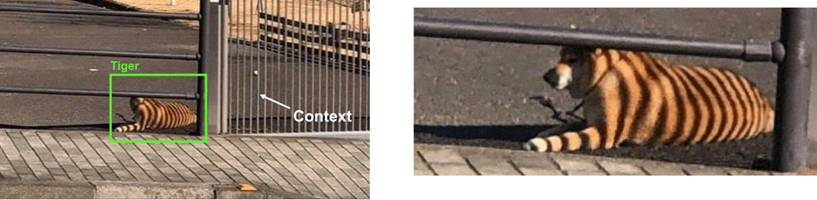
And that final challenge is Context. Humans are incredibly adept at using context to understand the world. We don’t just see objects in isolation; we see them within a scene, and that surrounding information heavily influences our perception. So what went wrong here? Here our model tend to latch onto local patterns, the stripping alone is enough to push our model prediction toward ‘tiger’. Our model didn’t sufficiently incorporate the fact this is on pavement, in front of a gate, and it turns out that it’s just someone’s small dog, and the tiger-stripes are the shadows cast by the iron bars of the gate across its fur. So, understanding and leveraging context is crucial for robust visual intelligence, but it’s also very difficult for current models to do this effectively. They often rely too heavily on local features and can miss the bigger picture or be fooled by misleading contextual cues.
Given all these hurdles, it should be clear that trying to write a program with explicit rules to identify, say, a ‘cat’ in all its possible manifestations and situations is an almost impossible task. We’d be writing if-else statements for years!
The three faces of a classifier
So now, we’re going to move on to a type of classifier, and arguably one of the most fundamental building blogs in machine learning and deep learning: the Linear Classifier. Linear classifier fall under what’s known as the Parametric Approach. This is a key distinction from K-Nearest Neighbors, which is a non-parametric method. In the parametric approach, we define a score function, let’s call it \(f(x, W)\), that map the raw input data(our image x) to class scores. The crucial part here is this \(W\). \(W\) represents a set of parameters or weights that the model uses. The “learning” process in a parametric model involves finding the optimal values for these parameters \(W\) using the training data. Once we’ve learned these parameters, we can effectively discard the training data itself! To make a prediction for a new image, we just need the learned parameters \(W\) and the function \(f\). This is very different from K-NN where we had to keep all the training data around.
Now, let’s get specific. What form does this function \(f(x,W)\) take for a linear classifier? It’s beautifully simple:
\[ f(x, W) = Wx \]
That’s it! It’s a matrix-vector multiplication. The result of \(Wx\) will be a vector of class scores. There’s one more small addition we typically make to this linear score function. We often add a bias term, \(b\) (though often we just write f(x,W) and assume W implicitly includes b, or b is handled separately).. So, the full form of our linear classifier’s score function becomes:
\[ f(x,W,b) = Wx + b \]
What is this bias \(b\)? It allows the score function to have some class-specific preferences that are independent of the input image \(x\). Think of it as shifting the baseline score for each class. For example, if in our training data, cats are just generally more common than airplanes, the bias term for “cat” might learn to be slightly higher, giving cats a bit of an advantage even before looking at the image pixels. It’s also common practice to sometimes absorb the bias term into the weight matrix \(W\) by appending a constant 1 to the input vector \(x\), and adding an extra column to \(W\) to hold the bias values. This just makes the notation a bit cleaner, \(f(x,W) = Wx\), but conceptually, it’s useful to think of \(W\) (the part that multiplies \(x\)) and \(b\) (the additive part) separately for a moment.
When it comes to interpreting a linear classifier, I think it’s easier for us to look at it from a few different perspectives
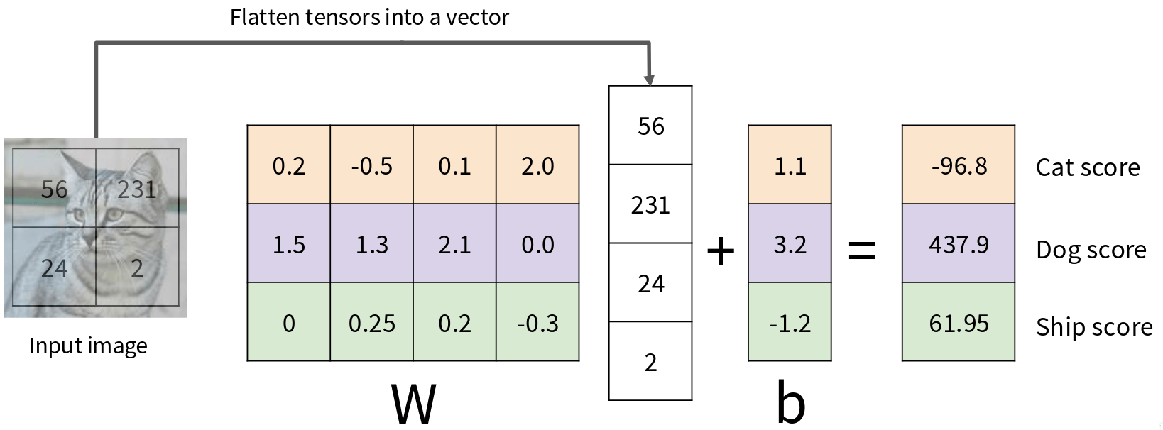
First is Algebraic Viewpoint. We need to produce 3 scores (one for cat, one for dog, one for ship). So our output should be a 3x1 vector. This means our weight matrix \(W\) must have dimensions [3 x 4] (3 rows for 3 classes, 4 columns to match the 4 pixels in \(x\)). And our bias vector \(b\) will be [3 x 1]. The first row of \(W\) are the weights for the “cat” class. The second row are the weights for the “dog” class. The third row are for the “ship” class. To get the scores, we perform the matrix multiplication \(Wx\) and then add \(b.\) So, for this input image and these particular weights \(W\) and biases \(b\), we get scores: Cat: -96.8, Dog: 437.9, Ship: 61.95. Based on these scores, which class would our linear classifier predict? It would predict “Dog,” because 437.9 is the highest score. The “learning” process, which we haven’t discussed yet, would be about finding values for \(W\) and \(b\) such that for an image that is a cat, the cat score is highest; for an image that is a dog, the dog score is highest, and so on.
Okay, we’ve seen the algebra. But can we get a more Visual Viewpoint of what these weights W actually represent? For CIFAR-10, each row of \(W\) is a vector of 3072 weights. Since our input \(x\) is an image, we can reshape each row of \(W\) back into a 32x32x3 image. What do these “images” corresponding to the rows of \(W\) look like?
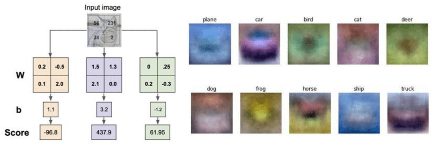
What the linear classifier is learning is essentially a single template for each class. When a new image comes in, it’s like the classifier is “matching” that input image against each of these 10 templates using a dot product. If the input image has, say, a lot of blue pixels in the regions where the “plane” template has blue pixels, and not many red pixels where the “plane” template has red pixels, that will contribute to a high score for the “plane” class. These templates are often very blurry and try to capture the “average” appearance of objects in that class. For example, cars can be many colors, but if there are more red cars in the training set, the “car” template might end up looking reddish. If planes are often pictured against a blue sky, the “plane” template might pick up on that blue. This also highlight a limitation: a linear learns only one template per class. But a class like “car” has many variations (red cars, blue cars, trucks, cars viewed from the side, car viewed from the front). A single template will struggle to capture this variability. It might learn a sort “average car”.
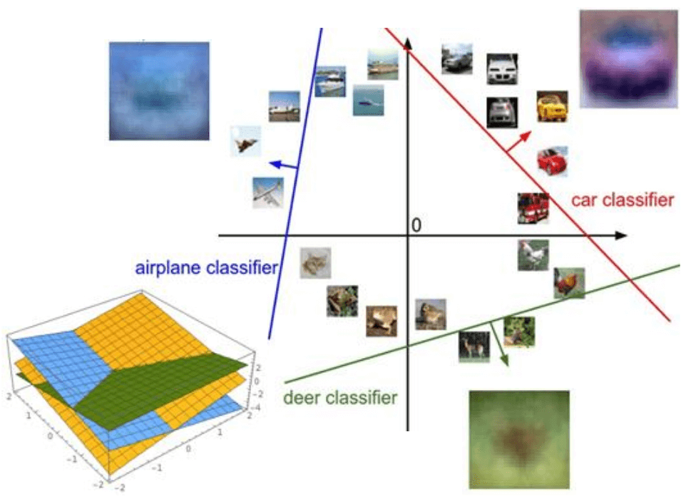
Finally let’s consider the Geometric Viewpoint. Our score function is \(s = Wx + b\). For each class c, the score for that class is \(s_c = W_c ⋅ x + b_c\), where \(W_c\) is the c-th row of \(W\). This is the equation of a line (or a hyperplane in higher dimensions). So, linear classifier is learning a set of hyperplane in the high-dimensional pixel space. Each hyperplane correspond to a class. The decision boundary between any two classes, say class \(i\) and class \(j\), occurs where their score are equal: \(W_ix + b_i = W_jx + b_j\). This equation also defines a hyperplane.
The 3D plot on the bottom left shows the actual score surfaces for three classes. Each colored plane represents the scores for one class as a function of a 2D input. The decision boundaries are where these planes intersect. You can see that the regions where one plane is highest correspond to the classification regions for that class. These regions are always convex polygons (or polyhedra in higher dimensions) for a linear classifier. So, geometrically, a linear classifier is carving up the high-dimensional input space using these hyperplanes. It’s trying to find orientations and positions for these hyperplanes such that most of the training examples for a given class fall on the “correct” side of their respective decision boundaries.
These three viewpoints – algebraic, visual (template matching), and geometric (hyperplanes) – all describe the same underlying mathematical operation \(Wx + b\). Understanding it from these different angles helps build a much richer intuition for what a linear classifier is doing, what it can learn, and also, importantly, what its limitations might be.
Hard cases for a linear classifier
There are scenarios where, no matter how you orient your lines (or hyperplanes in higher dimensions), you simply cannot perfectly separate the classes.
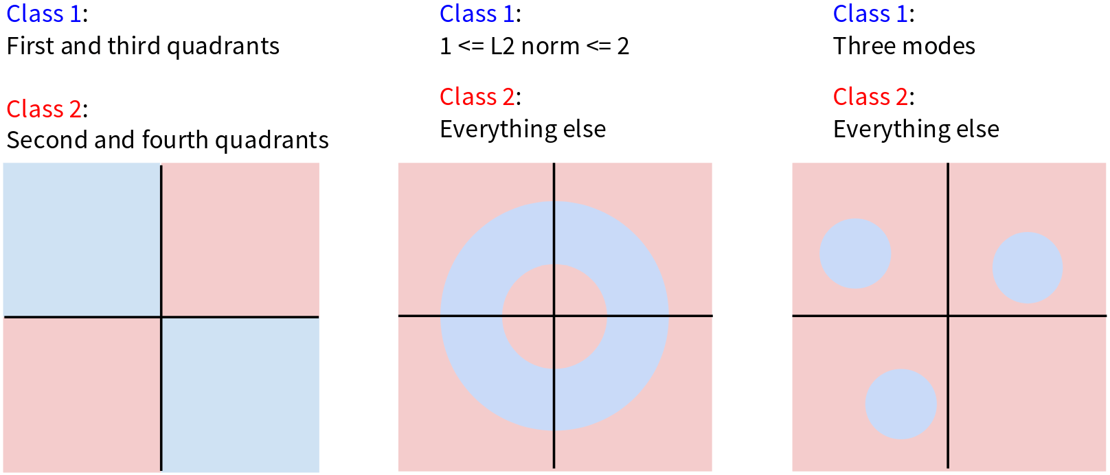
In case 1 we have the XOR problem where class 1 is in the first and third quadrants, class 2 is in the second and forth quadrants. Try to draw a single straight line, that separate the class 1 and class 2. You can do it! You’d need at least two lines, or a non-linear boundary. A linear classifier will fall here, it will make mistakes no matter what i places its decision boundary.
Case 2 is the donut problem, here, class 1 is an annulus or a ring – points whose L2 norm is between 1 and 2. Class 2 is everything else (inside the inner circle and outside the outer circle). Again, can you separate the blue ring from the pink regions with a single straight line? No. You’d need something like a circular boundary, which is non-linear.
Case 3 is Multiple modes, Class 1 consists of three distinct, separated circular regions. Class 2 is everything else. A single linear classifier tries to learn one template per class. If a class has multiple, well-separated “prototypes” or modes in the feature space, a linear classifier will struggle. It can’t draw a line to nicely encapsulate all three blue regions while excluding the pink. It might try to find a single hyperplane that does its best, but it will inevitably misclassify many points.
Choose a good W
So, given that we have this linear score function \(f(x,W) = Wx + b\), and we understand its capabilities and limitations, the central question becomes: How do we choose a good \(W\) (and \(b\))? We need a systematic way to 1) define a loss function (or cost function or objective function). This function will take our current \(W\) and \(b\), run our classifier on the training data, look at the scores it produces, and tell us how “unhappy” we are with those scores. A high loss means our \(W\) and \(b\) are bad (producing scores that lead to incorrect classifications or low confidence in correct classifications). A low loss means our \(W\) and \(b\) are good. 2) Once we have this loss function, we need to come up with a way of efficiently finding the parameters (\(W\) and \(b\)) that minimize this loss function. This is an optimization problem. We want to search through the space of all possible \(W\)’s and \(b\)’s to find the set that makes our classifier perform best on the training data, according to our loss function.
More formally, we are given a dataset of \(N\) training examples:
\[ { (x_i, y_i) }_{i=1}^{N} \]
Where \(x_i\) is an image (our input vector) and \(y_i\) is its true integer label (e.g., 0 for cat, 1 for car, 2 for frog). Typically, the total loss over the entire dataset, \(L\), is the average of the losses computed for each individual training example:
\[ L = \frac{1}{N} \sum_i L_i(f(x_i, W), y_i) \]
Here:
- \(f(x_i, W)\) are the scores our current classifier (with weights \(W\)) produces for the i-th training image \(x_i\).
- \(y_i\) is the true label for that i-th training image.
- \(L_i\) is the loss function calculated for that single i-th example. It takes the predicted scores and the true label and tells us how bad the prediction was for that one example.
- We sum these individual losses \(L_i\) over all \(N\) training examples and then divide by \(N\) to get the average loss
Our goal will be to find the \(W\) that minimizes this total loss \(L\). Now, the crucial piece we still need to define is: what exactly is this \(L_i\) function? How do we take a vector of scores and a true label and turn that into a single number representing the loss for that example? There are several ways to do this, and we’ll look at a very common one for classification next: the Softmax classifier (which uses cross-entropy loss), and also the SVM (hinge) loss.
Softmax classifier
The core idea behind the Softmax classifier is that we want to interpret the raw classifier scores as probabilities. Our linear classifier \(s = f(x_i, W)\) produces these raw scores. For example our cat image example, we had scores: Cat: 3.2, Car: 5.1, Frog: -1.7. These are just arbitrary real numbers. They could be positive, negative, large, small. They don’t look like probabilities, which should be between 0 and 1 and sum to 1. The Softmax function is what allows us to convert these raw scores into a valid probability distribution over the classes. The formula for the probability of the true class \(k\) given the input image \(x_i\) (and our weights \(W\)) is:
\[ P(Y = k | X = x_i) = \frac{e^{s_k}}{\sum_j e^{s_j}} \]
Where:
- \(s_k\) is the raw score for class \(k\) (e.g., 3.2 for cat).
- \(s_j\) are the raw scores for all classes \(j\) (cat, car, frog).
- We exponentiate each score (\(e^{s_k}\)). This makes all the numbers positive, which is good for probabilities.
- Then we normalize by dividing by the sum of all these exponentiated scores. This ensures that the resulting probabilities for all classes sum to 1.
The raw scores s that go into the Softmax function (our 3.2, 5.1, -1.7) are often called logits or unnormalized log-probabilities. The term “logit” comes from logistic regression, of which Softmax is a generalization to multiple classes
Okay, so we’ve used the Softmax function to get a probability distribution over the classes for a given input image \(x_i.\) Now, how do we define the loss \(L_i\) for this single example? If the true class for our example image (the cat) is y_i (let’s say “cat” is class 0), then the loss for this example is defined as the negative log probability of the true class:
\[ L_i = -\log{P(Y = y_i|X = x_i)} \]
Why this particular form for the loss? Probabilities \(P\) are between \(0\) and \(1\). \(log(P)\) will be negative (or \(0\) if \(P=1\)). If the probability of the true class is very high (close to \(1\), e.g., \(P=0.99\)), then \(log(P)\) is close to \(0\), and \(-log(P)\) is also close to \(0\) (a small loss, which is good!). If the probability of the true class is very low (close to \(0\), e.g., \(P=0.01\)), then \(log(P)\) is a large negative number, and \(-log(P)\) will be a large positive number (a high loss, which is bad!). So, this \(-log(P_true_class)\) loss function does what we want: it penalizes the model heavily if it assigns low probability to the correct answer, and penalizes it very little if it assigns high probability to the correct answer. Minimizing this loss will push the model to make the probability of the true class as close to \(1\) as possible. This approach also known as Maximum Likelihood Estimation (MLE). We are choosing the parameters \(W\) to maximize the likelihood (or equivalently, the log-likelihood) of observing the true labels \(y_i\) given the input data \(x_i.\) Taking the negative log-likelihood turns it into a loss minimization problem.
We can also think about this loss from an information theory perspective. The “correct probabilities” for our cat image would be: Cat: 1.00, Car: 0.00, Frog: 0.00. This is a probability distribution where all the mass is on the true class. Let’s call this target distribution \(P\). Our Softmax classifier produced the distribution Q: Cat: 0.13, Car: 0.87, Frog: 0.00. The loss function we are using, \(-log P(Y=y_i | X=x_i)\), is actually equivalent to the Kullback-Leibler (KL) divergence between the true distribution P (which is 1 for the correct class and 0 otherwise) and the predicted distribution Q from our Softmax. The KL divergence \(D_KL(P || Q)\) measures how different the distribution \(Q\) is from the distribution \(P\). It’s defined as \(\sum_y P(y)\log\frac{P(y)}{Q(y)}\). When P is a one-hot distribution (1 for the true class \(y_i\), \(0\) elsewhere), this simplifies to \(-logQ(y_i)\), which is exactly our loss function!
So, the loss \(L_i = -log P(Y=y_i | X=x_i)\) for a Softmax classifier is often called the Cross-Entropy loss between the true distribution (one-hot encoding of the correct label) and the predicted probability distribution from the Softmax.
\[ H(P,Q) = - \sum_y P(y) log Q(y) \]
When \(P\) is one-hot, \(P(y)\) is \(1\) for the true class \(y_i\) and \(0\) otherwise. So, the sum collapses to a single term: \(-1 log Q(y_i) = -log Q(y_i)\).
So, whether you think of it as maximizing the log-likelihood of the correct class, or minimizing the KL divergence, or minimizing the cross-entropy between the true and predicted distributions, it all leads to the same loss function for the Softmax classifier: \(L_i = -log(\text{probability\_of\_true\_class})\). This is a cornerstone loss function for classification problems in deep learning. The overall loss for the dataset, L, would then be the average of these L_i’s over all training examples. Our goal is to find the W that minimizes this total cross-entropy loss.
So, just to recap:
- We start with raw scores \(s = f(x_i, W)\) from our linear classifier.
- We want to interpret these as probabilities, so we use the Softmax function: \(P(Y = k | X = x_i) = \frac{e^{s_k}}{\sum_j e^{s_j}}\). This gives us a probability for each class \(k\).
- Our goal is to maximize the probability of the correct class \(y_i\).
- The loss function \(L_i\) for a single example is the negative log probability of the true class: \(L_i = -log P(Y = y_i | X = x_i)\).
Putting it all together, we can write the loss for a single example \(x_i\) with true label \(y_i\) and scores \(s_j\) (where \(s_j\) is the score for class \(j\)) directly as:
\[ L_i = -log ( \frac{e^{ s_{y_i} }}{\sum_j e^{ s_j }} )\]
Here, \(s_yi\) is the score for the true class \(y_i\). This formula combines the Softmax calculation and the negative log operation into one expression for the loss. Minimizing this \(L_i\) will push the score of the correct class \(s_yi\) to be high relative to the scores of the other classes \(s_j\).
Now, let’s think about some properties of this Softmax loss \(L_i\). Two good questions to consider: What is the minimum and maximum possible Softmax loss \(L_i\)? And at initialization, our weights W are typically small random numbers. So, the initial scores \(s_j\) for all classes will be approximately equal (and close to zero). What will the Softmax loss \(L_i\) be in this scenario, assuming there are C classes?
Answer for the first question: Minimum possible loss, the loss is \(L_i = -log(\text{P\_correct\_class})\). To minimize \(L_i\), we need to maximize P_correct_class. The maximum possible probability for the correct class is 1 (i.e., the classifier is 100% certain and correct). If \(P\_correct\_class = 1\), then \(log(1) = 0\), so \(L_i = -0 = 0\). Thus, the minimum possible Softmax loss is 0. This occurs when the model perfectly predicts the true class with probability 1. Maximum possible loss, to maximize \(L_i\), we need to minimize P_correct_class. The minimum possible probability for the correct class is something very close to 0 (it can’t be exactly 0 because of the exponentiation, but it can be arbitrarily small if the score for the correct class is very, very negative relative to other scores). As P_correct_class approaches 0 from the positive side, log(P_correct_class) approaches negative infinity. Therefore, \(-log(\text{ P\_correct\_class })\) approaches positive infinity. So, the Softmax loss can, in theory, go to infinity if the model is extremely confident in a wrong class and assigns vanishingly small probability to the true class.
Now for question 2: If all \(s_j\) are approximately equal (say, \(s_j \approx s\_constant\)), then \(e^{s_j}\) will also be approximately equal for all \(j\). The probability for any given class k will be:
\[ P(Y=k | X=x_i) = \frac{e^{s_k}}{\sum_j e^{s_j}} \]
Since all \(e^{s_j}\) are roughly the same, let’s say \(e^{s\_constant}\), the sum in the denominator will be \(C e^{s\_constant}\). So, \(P(Y=k | X=x_i) \approx \frac{e^{s\_constant}}{C e^{ s\_constant }} = \frac{1}{C}\).
This makes intuitive sense: if the classifier has no information yet (all scores are equal), it should assign an equal probability of 1/C to each of the C classes. This is a uniform distribution. Now, the loss for any example \(x_i\) (regardless of its true class \(y_i\), since the probability assigned to every class is 1/C) will be:
\[ L_i = -log(P\_correct\_class) = -log(\frac{1}{C}) \]
Using the logarithm property \(log(\frac{1}{C}) = log(1) - log(C) = 0 - log(C) = -log(C)\). So, \(L_i = -(-log(C)) = log(C)\). Therefore, at initialization, when the classifier is essentially guessing uniformly, the Softmax loss per example will be approximately \(log(C)\), where \(C\) is the number of classes. For example, if we have \(C = 10\) classes (like in CIFAR-10), then the initial loss we expect to see is \(L_i = log(10)\) (natural logarithm of 10), which is approximately 2.3. This is a very useful “sanity check”! When you’re implementing a Softmax classifier and you initialize your weights, if you compute the loss on your first batch of data and it’s wildly different from \(log(C)\), you might have a bug somewhere in your loss calculation or your Softmax implementation. For CIFAR-10, you should see an initial loss around 2.3. If you see a loss of, say, 20 or 0.01 at the very start, something is likely wrong.
Multiclass SVM loss
Alright, so we’ve seen the Softmax classifier and its cross-entropy loss. Now, let’s turn to the other major type of loss function for linear classifiers: the Multiclass SVM loss, also known as the hinge loss. The Multiclass SVM loss has a different philosophy than Softmax. The SVM wants the score of the correct class \(s_{y_i}\) to be greater than the score of any incorrect class \(s_j\) (where \(j ≠ y_i\)) by at least a certain fixed margin, which is commonly denoted by \(\Delta\) and often set to 1. Here’s the form of the loss L_i for a single example:
\[ L_i = \sum_{j \ne y_i} \begin{cases} 0 & \text{if } s_{y_i} \geq s_j + 1 \\ s_j - s_{y_i} + 1 & \text{otherwise} \end{cases} = \sum_{j \ne y_i} \max(0, s_j - s{y_i} + 1) \]
So, for each training example, we sum up these margin violation penalties over all incorrect classes. If all incorrect classes have scores that are at least \(\Delta\) less than the score of the correct class, then \(L_i\) will be 0 for that example.
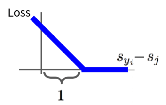
Let’s visualize what one term \(\max(0, s_j - s_{y_i} + 1)\) of this loss looks like. The x-axis here is representing \(s_{y_i} - s_j\), which is the difference between the score of the correct class and the score of one particular incorrect class \(j\). The SVM loss wants the score of the correct class \(s_{y_i}\) to be greater than the score of an incorrect class \(s_j\) by at least the margin \(\Delta\) (which is 1 in our plot). So, if \(s_{y_i} - s_j \geq 1\), meaning the correct score is already beating the incorrect score by the desired margin then the loss for that pair is 0. You can see the loss function is flat at 0 on the right side of the plot, where \(s_{y_i} - s_j \geq 1\). The SVM doesn’t care how much better the correct score is, as long as it’s better by at least the margin. It doesn’t try to push the correct score infinitely higher or the incorrect scores infinitely lower, unlike Softmax which is never fully satisfied. However, if \(s_{y_i} - s_j \lt 1\) (i.e., the margin is violated), then the loss becomes positive. The loss increases linearly as the difference \(s_{y_i} - s_j\) gets smaller (or more negative, meaning \(s_j\) is much larger than \(s_{y_i}\)). This is the hinge shape - zero loss if the margin is met and then a linear penalty for violations. The total \(L_i\) for an example is the sum of these hinge losses over all incorrect classes \(j\). This encourages the score of the true class \(y_i\) to stand out from all other incorrect class scores by at least \(\Delta\). This is a fundamentally different way of thinking about loss compared to Softmax. Softmax wants to correctly estimate the probability distribution; SVM wants to find a decision boundary that separates classes with a good margin.
So what is the min/max possible SVM loss L_i? Minimum possible loss, if all margins are satisfied (i.e., for all incorrect classes \(j\), \(s_{y_i} \geq s_j + \Delta\)), then every term in the \(\sum \max(0, s_j - s_{y_i} + \Delta)\) will be 0. So, the minimum SVM loss \(L_i\) is 0. Maximum possible loss, if the score for the correct class \(s_{y_i}\) is extremely negative, and scores for incorrect classes \(s_j\) are very positive, then \(s_j - s_{y_i} + \Delta\) can become arbitrarily large and positive for each incorrect class. Since we sum these terms, the total \(L_i\) can go to positive infinity.
At initialization, \(W\) is small, so all scores \(s_j \approx 0\). What is the loss \(L_i\), assuming \(C\) classes? If all \(s_j \approx 0\) (including \(s_{y_i} \approx 0\)), then for each of the \(C-1\) incorrect classes j, the term is:
\[s_j - s_{y_i} + \Delta ≈ 0 - 0 + \Delta = \Delta\]
So, \(\max(0, \Delta)\) is just \(\Delta\) (assuming our margin \(\Delta\) is positive, e.g., \(\Delta=1\)). We sum this \(\Delta\) over all \(C-1\) incorrect classes. Therefore, \(L_i ≈ (C-1) \Delta\). If \(\Delta=1\), then the initial loss \(L\) is approximately \(C-1\). For CIFAR-10 with \(C=10\) classes and \(\Delta=1\), the initial SVM loss per example would be around 9. This is another good sanity check for your implementation. If you see an initial SVM loss far from \(C-1\), you might have an issue.
What if we used a squared term for the loss: \(L_i = \sum_{j \neq y_i} \max(0, s_j - s_{y_i} + \Delta)^2\)? This is known as the squared hinge loss (or L2-SVM). The standard (L1) hinge loss \(\max(0, margin\_violation)\) penalizes any violation linearly. Every unit of margin violation contributes equally to the loss. The squared (L2) hinge loss \(\max(0, margin\_violation)^2\) penalizes larger violations much more heavily than smaller ones due to the squaring. It’s more sensitive to outliers or examples that are very wrong. This can sometimes lead to different solutions. Both have been used, though the L1 hinge loss is perhaps more standard for the classic SVM. The L2 version is smoother (differentiable even when the margin violation is zero, though the max(0,…) still introduces a non-differentiability point when the argument to max is exactly zero), which can sometimes be beneficial for certain optimization algorithms.
Here’s a python function that calculates the SVM loss for a single example x with true label y, given weight W.
def L_i_vecterized(x, y, W):
1  scores = W.dot(x)
2  margins = np.maximum(0, scores - score[y] + 1)
3  margins[y] = 0
  loss_i = np.sum(margin)
return loss_i- 1
- calculate scores
- 2
- then calculate the margins \(s_j - s_{y_i} + 1\)
- 3
- only sum \(j\) is not \(y_i\) so when \(j = y_i\), set to zero
This is a nice, compact vectorized implementation. To get the loss for a whole batch of data, you’d typically loop over your batch, call this function for each example, and then average the results.
SVM is a margin-based loss. Softmax is a probabilistic loss that cares about the full distribution. In practice, both are widely used, and sometimes one might perform slightly better than the other depending on the dataset and task, but often their performance is quite similar when used in deep networks. The choice can also come down to whether you explicitly need probability outputs from your model.