A brief history of computer vision and deep learning

“A split scene: on one side, an old master painter (think Da Vinci) painting a realistic portrait, and on the other, a futuristic robot painting a digital image using code or neural networks as its brush strokes”, generated by DALL·E 3

My goal over the next ten weeks or so is to have a deep, foundational understanding of the principles and practices that are driving the state-of-the-art in visual intelligence. So to begin our journey, I find it useful to first situate what we will be studying within a broader intellectual landscape. We can start with the most encompassing field: Artificial Intelligence.

Our place on the AI map

AI is the grand, overarching ambition. It’s the quest to build machines that can perform tasks that have historically required human intelligence (tasks like reasoning, planning, and perception). It’s a field with a long and rich history, full of profound philosophical questions and formidable engineering challenges.

Where are we at? A broad view of the field of AI - Image inspired by Justin Johnson

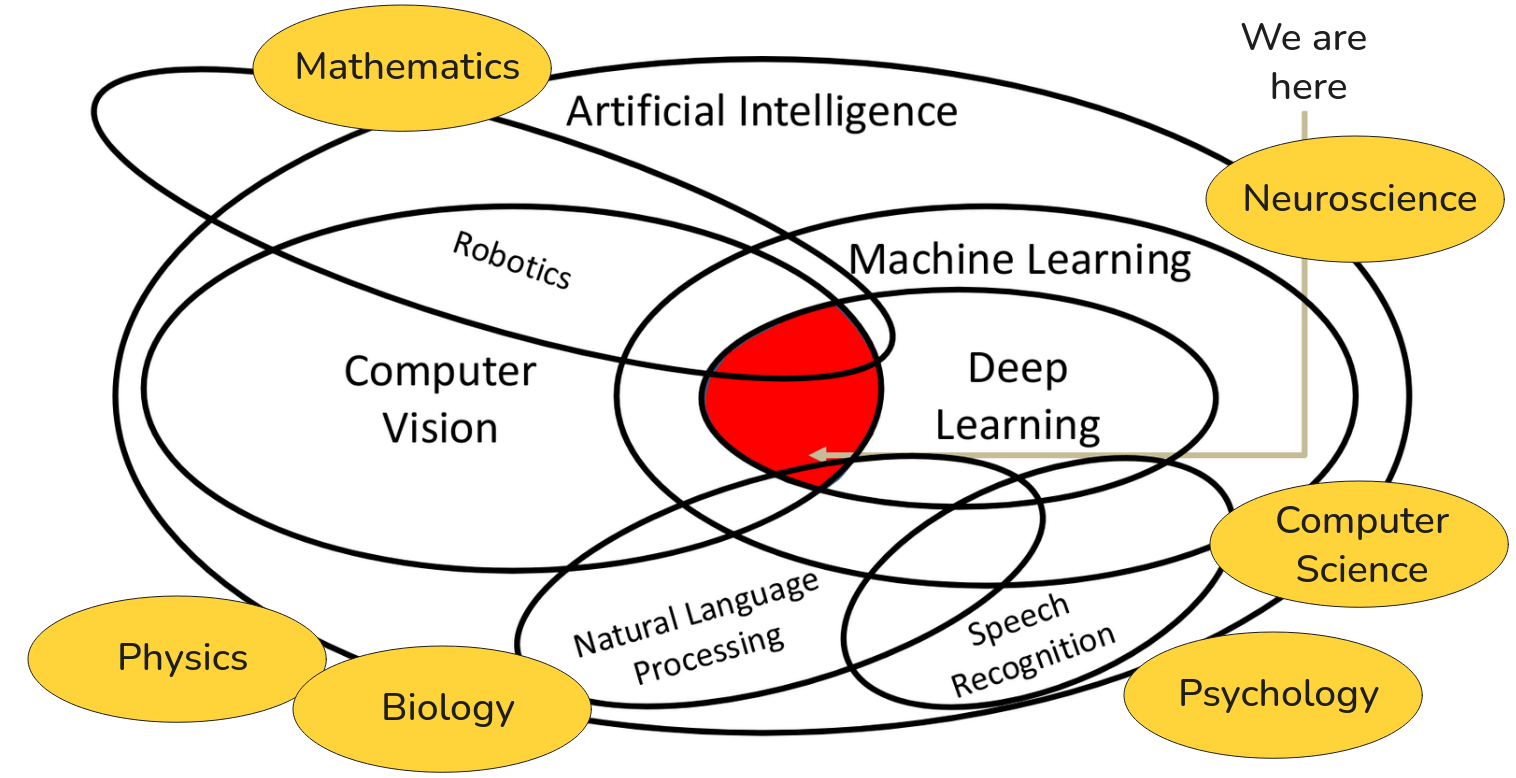
Now, AI is an enormous domain. Within it, we can delineate several major sub-disciplines. Two of the most significant are Machine Learning and Computer Vision. Machine learning is a specific approach to achieving AI. Instead of explicitly programming a machine with a set of handcrafted rules to solve a task, the machine learning paradigm is to develop algorithms that allow machine to learn the rules by itself, by analyzing data. This shift from rule-based system to data-driven system is a fundamental concept that we will return to again and again. Then we have Computer Vision. This is the scientific and engineering discipline dedicated to a different goal: enabling machines to see. That is, to take in visual information from the world, from images, from video and to derive understanding from it. These two fields have a significant and ever-growing intersection. While there exists a body of classical computer vision work that does not rely on machine learning, think of the techniques from computational geometry or signal processing but the most powerful and prevalent methods in modern computer vision are fully rooted in machine learning.

Now let’s zoom in one level deeper. Within Machine Learning, a particular subfield has emerged over the last decade or so that has completely revolutionized the landscape. And that is Deep Learning. Deep learning is a specific class of machine learning algorithms. The defining characteristic is the use of neural networks with many layers, hence “deep” networks. These architectures, as we will go into great detail, have proven to be exceptionally effective at learning intricate patterns and hierarchical representations from vast amounts of data.

This brings us to the core focus of our discussion. The intersection of Deep Learning and Computer Vision. The red area on the diagram above is where we will spend our time. Our objective is to understand and implement deep learning architectures and methodologies that are purpose-built to solve computer vision problems. This convergence is responsible for nearly all of the dramatic breakthroughs in visual perception you may have seen in recent years.

However, it’s crucial to understand that while our focus is on vision, deep learning is not exclusively a tool for computer vision. It is a general-purpose computational paradigm that has had a similar transformative impact on other fields of AI. For example, another major subfield is Natural Language Processing, or NLP, which deals with enabling computers to understand and generate human language. And a closely related field is Speech Recognition, which focuses on converting spoken language into text. Both NLP and Speech have been fundamentally reshaped by the application of deep learning models.

We can further expand our map to include fields like Robotics. Robotics is an inherently integrated discipline. A truly autonomous robot must perceive its environment (which is a core computer vision problem) and then decide how to act, which often evolves from experience(a machine learning problem). Therefore, robotics draws heavily from both computer vision and machine learning and increasingly, deep learning is the unifying methodology.

Mathematics, particularly linear algebra, probability, and calculus, provides the formal language and the core tools we use to define and optimize our models. Neuroscience and Psychology provide the biological inspiration for our network architectures and offer insights into the nature of intelligence itself. We also have Physics because we need to understand optics and image formation and how images are actually formed. We need to understand Biology and Psychology how the animal brain physically sees and processes visual information. And of course, all of this is built upon the substrate of Computer Science which gives us the algorithms, data structures, and high-performance computing systems necessary to make these computationally intensive ideas a reality.

Finally, it’s imperative to recognize that none of these fields exists in a vacuum. They are built upon and draw inspiration from a wide array of fundamental scientific disciplines. So while we will live in that red intersection of deep learning and computer vision, I want you to maintain this broader perspective. The work we do here connects to a rich and interdisciplinary tapestry of human knowledge.

Why vision? From first eye to billion cameras

Alright, so that gives you the sense of the intellectual landscape so let’s begin with the history. And to truly appreciate the motivation of our field i find it instructive to go back… quite a long way.

Early multicellular life and the dawn of vision. All images from Wikipedia / CC‑BY. Left: Burgess Shale trilobite fossil preserving antennae and legs. Top right: Dickinsonia costata, a quilted Ediacaran organism of unknown affinity. Bottom right: Artistic reconstruction of Opabinia, the five‑eyed Cambrian critter that helped ignite interest in the Cambrian explosion.

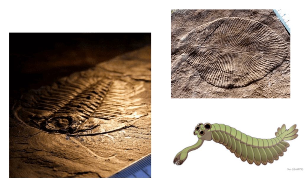
Roughly 540 million years ago, our planet experienced a period of unprecedentedly rapid diversification of complex, multicellular life. This is known as the Cambrian Explosion. And a leading scientific hypothesis for what acted as the primary catalyst for this “big bang” of evolution… was the advent of vision.

The development of the first primitive eyes created an enormous new set of evolutionary pressures. For the very first time, organisms could actively hunt, evade predators, and navigate their environment with a richness of information that was previously unimaginable. In a very real sense the ability to see changed the rules of life on Earth, and may have been the driving force behind the development and much of the biological complexity we see today.

Octopus camera-type eye, insect compound eye, chameleon turret eye, human binocular eye.

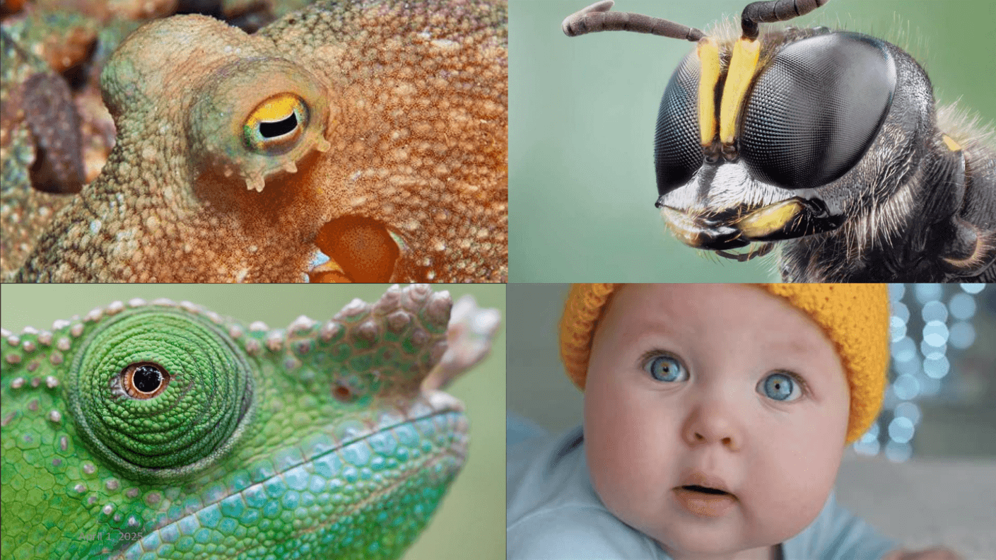
And the legacy of that ancient innovation is all around us. Vision is a powerful example of convergent evolution. It has been independently invented by nature dozens of times across the tree of life. From the compound eyes of insects, which excel at detecting motion, to the incredibly sophisticated camera-like eyes of octopus, to the remarkable independently moving eyes of a chameleon… and of course, to our own visual system. The fact that evolution has arrived at the solution of “the eye” so many times underscores it profound utility as a mechanism for interacting with the world

For most of history vision was a purely biological phenomenon. But humanity has long been obsessed with capturing what we see, with creating an external record of our vision perception.

The Camera Obscura. Top right: first published picture of camera obscura, in Gemma Frisius’ 1545. Bottom right: Leonardo da Vinci, 16th Century AD. Left: camera obscura in Encyclopedia, 18th Century (all images from From Wikipedia, the free encyclopedia)

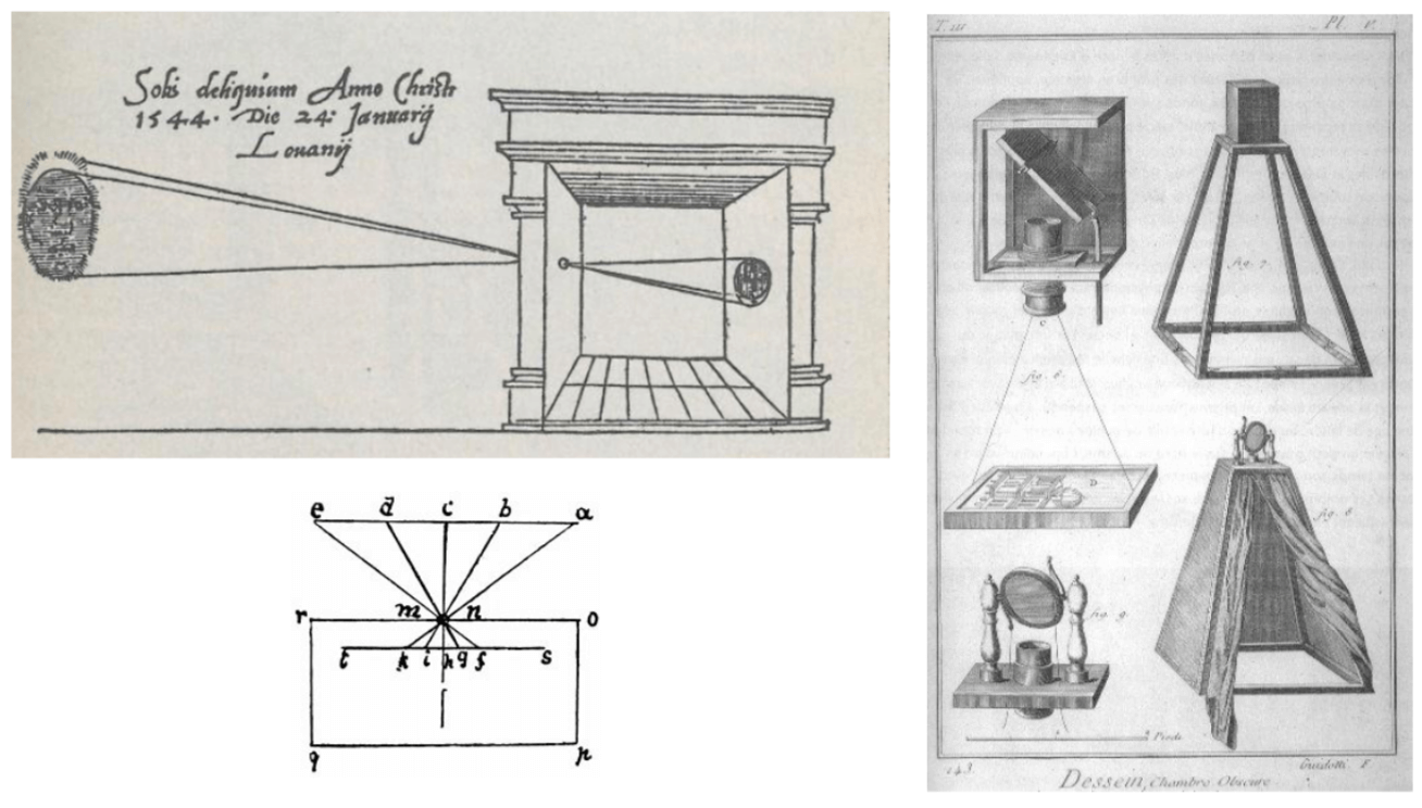
This quest leads us to one of the most foundational principles in the history of imaging: The Camera Obscura, which is Latin for “dark chamber”. As early as the 16th century, and with principles understood even in antiquity, scholars and artists recognized that if you have a darkened enclosure with a small aperture, an inverted image of the external scene is projected into the opposite wall. This is the fundamental principle upon which all photography and even modern cameras is built. It represents the first critical step in humanity’s attempt to externalize the scene of sight.

Now, if we fast-forward from the simple pinhole in a dark room to the 21st century, the consequence of that is… staggering.

Computer vision is now everywhere. First row, left to right: [1], [2], [3], [4]. Second row, left to right: [1], [2], [3], [4]. Third row, left to right: [1], [2], [3], [4]

The reason we have a field called computer vision today is, in large part, because the sensors of vision (cameras) are utterly ubiquitous. They are in our pocket, in our cars, in our homes, attached to drones, flying through the air, and even roving the surface of other planets.

The proliferation of inexpensive, high-resolution digital cameras has resulted in an unprecedented deluge of visual data. More images are now captured every two minutes than were captured in the entire 19th century. This vast sea of pixels is the raw material, the fuel, that powers the deep learning models we will talk about a lot.

So this brings us to a critical question. We have this deep, biological imperative for vision, and we have this modern technological reality of ubiquitous cameras generating near-infinite data. Given this perfect storm of motivation and raw material… how did the scientific engineering discipline of Computer Vision actually come to be? Where did we, as a field, come from?

Neuroscience lights the way

The story often begins not in computer science but in neuroscience. In 1959, two neuroscientists, David Hubel and Torsten Wiesel, conducted a series of now-famous experiments for which they would later win the Nobel Prize. They sought to understand the architecture of the mammalian visual system. They did this by inserting microelectrodes into the primary visual cortex—the first cortical area to receive input from the eyes of an anesthetized cat. They then presented the cat with very simple visual stimuli on a screen—things like bars of light, dots, or oriented edges.

Hubel & Wiesel’s classic 1959 cat–visual‑cortex experiment (image inspired by Justin Johnson)

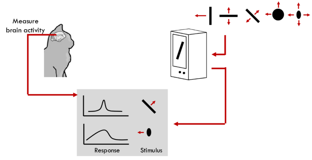
What they discovered was remarkable. They found that individual neurons in the brain region were not responding to complex concepts like “a mouse” or “a food bowl”. Rather, they were highly specialized feature detectors. They identified two principal classes of cells. First, simple cells. A given simple cell would fire vigorously as shown in the top response graph, only when a bar of light with a very specific orientation appeared at a very specific location in the visual field. If the orientation was wrong, or if the stimulus was just a dot, the neuron remained silent. Then they found complex cells. These cells also respond to oriented edges, but they were invariant to the precise location of that edge within their receptive field. As you can see on the diagram, the bar can move, or translate, and the complex cell continues to fire. Many were also tuned to the direction of motion.

This discovery was profoundly influential. It provided the first biological evidence for a hierarchical visual processing system. Where the initial stages are dedicated to detecting simple, local features like oriented edges. This idea of building up complex recognition from a hierarchy of simple feature detectors is a cornerstone of modern computer vision, and as we will see, it is the fundamental architectural principle behind convolutional neural networks.

Just a few years later, inspired in part by this new understanding of biological vision, the field of computer vision had its genesis. Larry Robert’s 1963 PhD thesis MIT is widely considered to be the seminal work.

Roberts’s 1963 “block world” vision pipeline (image from epicsysinc)

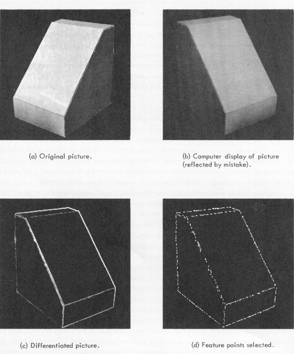
His system aimed to solve what seems like a simple problem: understanding the 3D geometry of simple “block world” scenes from a single 2D image. His approach was a pipeline. First take the original image. Second compute a “differentiated picture” which is a computational method for finding sharp changes in intensity in other words, an edge detector. This is a direct computational analog of what Hubel and Wiesel’s simple cell was doing. Finally, from this edge map, he would select feature points like corners and junctions and use geometric reasoning to infer the 3D shape. This was the start: a non-learning, rule-based system that decomposed vision into a series of explicit steps: find edges, find junctions, infer geometry.

This early success bred a great deal of optimism. So much so that in 1966, a group at MIT, led by Seymour Papert, proposed what is now famously known as “The Summer Vision Project”. The idea was, now we’ve got digital cameras, now they can detect edges, and Hubel and Wiesel told us how the brain works so basically what he wanted to do is hang a couple undergrads put them to work over the summer and after the summer we show it we should be able to construct a significant portion of visual system. The ambition was, in essence, to largely solve the problem of vision in a single summer by breaking it down into sub-problems. This, of course, turned out to be a profound underestimation of the problem’s difficulty. Now it’s clearly the computer vision was not solved and nearly 60 years later we’re still plugging away trying to achieve this what they thought they could do it in a summer with few undergrads. But it speaks to the excitement and perceived tractability of the field in its infancy.

Following this period of excitement and subsequent realization of the problem’s true depth, the field entered a phase of more systematic, theoretical thinking. The most influential of this era was David Marr.

Stages of Visual Representation, David Marr, 1970s. Bottom right: Recognition via Parts (1970s)

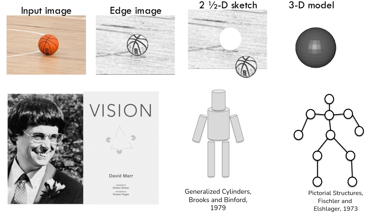
In the 1970s, Marr proposed a comprehensive framework for how a visual system should be structured. He argued for a staged, bottom-up pipeline. You start with an input image just an array of pixel intensities. The first stage is to compute what he called the Primal Sketch. This is a representation of 2D image structure, identifying primitive elements like zero-crossing, edges, bars, and blobs. Again, you see the direct intellectual lineage from Hubel and Wiesel. From the Primal Sketch, the system would then compute the 2.5-D Sketch. This is a viewer-centric representation that captures local surface orientation and depth discontinuities. It’s not a full 3D model, but rather a map of how surfaces are angled relative to the observer. Finally from the 2.5-D Sketch, the system would construct a full, object-centered 3-D Model Representation, describing the shapes and their spatial arrangement in a way that is independent from the viewpoint. This framework was immensely influential and guided vision research for many years.

Marr’s ideas spurred a great deal of research into how one might actually represent these 3D models. One popular idea from the 1970s was “Recognition via Parts”. One formulation of this was the idea of Generalized Cylinders proposed by Brooks and Binfold. The concept is to represent complex objects as a composition of simple, parameterized volumetric primitives like cylinders. A human figure can be modeled as an articulated collection of these cylinders. Another related idea was that of Pictorial Structure, from Fischler and Elshlager. Here, an object is represented as a collection of parts arranged in a deformable configuration, like nodes, connected by springs. This captures both the appearance of the parts and their plausible spatial relationships. Both of these are instantiations of the core idea that object recognition proceeds by identifying constituent parts and their arrangement.

Recognition via Edge Detection (1980s) - Edge detection algorithms by John Canny, 1986

Throughout the 1980s, much of the field’s energy was focused on perfecting the very first stage of Marr’s pipeline: edge detection. The thinking was that if we could just produce a perfect line drawing of the world from an image, as you see on the right, the subsequent steps of recognition would be much more tractable. This led to seminal work on edge detection algorithms, most famously by John Canny in 1986, whose algorithm is still baseline today, and also by David Lowe, whom we will encounter again later. The field became very good at turning images of things like those razors into learn edge maps.

Now, zooming out to the broader context of artificial intelligence during this period… something important was happening. The field was entering what became known as an “AI winter”. The massive enthusiasm and, critically, the government funding for AI research began to dwindle. This was largely the dominant paradigm of the time, so-called “Expert Systems” which tried to encode human expertise in vast, handcrafted rule-bases had failed on their very grandiose promise. However, this didn’t mean that research stopped. Instead, the subfield of AI, like computer vision, NLP, and robotics, continued to mature. They grew into more distinct disciplines, focusing on their own specific problems and developing their own specialized techniques, often with less of the grand, unifying ambition of the early AI pioneers.

But in the meantime.. while this entire arc of “classical” computer vision was unfolding, from Hubel and Wiesel to Marr to edge detector… another set of ideas, also with roots in neuroscience and cognitive science, was developing in parallel. And it is this other thread of history that will ultimately lead us to the “deep learning” part.

Learning to find faces in a crowd

Throughout the 1970s and 80s, cognitive scientists were conducting experiments that revealed just how complex and sophisticated the human system truly is, often in ways that these early models couldn’t account for.

Irving Biederman’s experiment in the early 1970s.

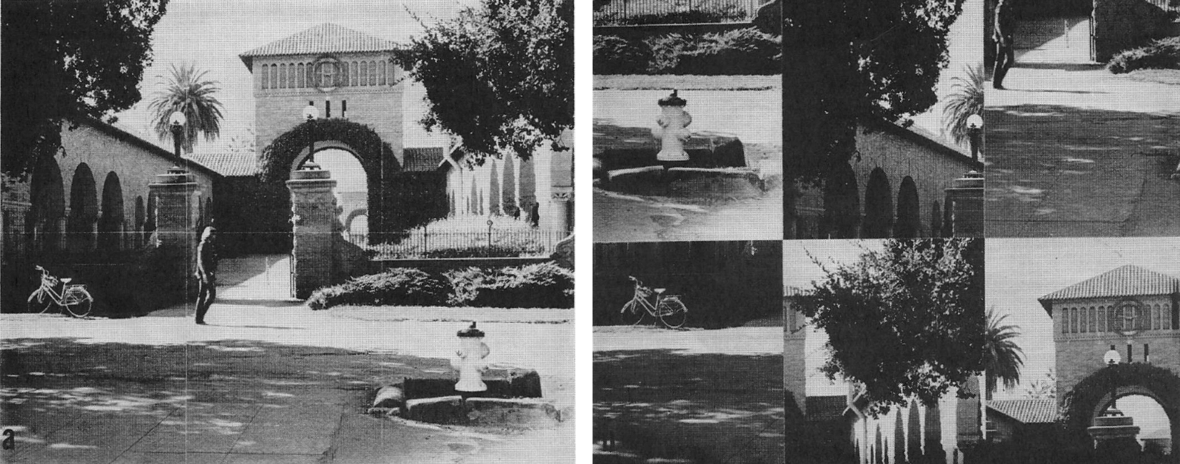
One such piece of work comes from Irving Biederman in the early 1970s. He represented subjects with images like the one you see on the left—a coherent, real-world scene. Unsurprisingly, people can recognize this scene and its constituent objects almost instantaneously. But then he would show them an image like the one on the right, which contains the exact image patches, but jumped into a non-sensical configuration. Recognition of the individual objects in this jumbled scene is significantly slower and more difficult. This simple but elegant experiment demonstrates a crucial point: our visual system doesn’t just recognize isolated parts. It relies heavily on the global context and the plausible spatial arrangement of those parts. The “whole” is more, and is processed differently than, the sum of its parts. This posed a significant challenge to a purely bottom-up, part-based recognition pipeline.

Another line of inquiry focused on the sheer speed of human vision. A common experimental paradigm used to study this is called Rapid Serial Visual Perception, or RSVP. The setup is simple: a subject fixates on a cross at the center of a screen, and images are flashed in very rapid succession often for only a few tens of milliseconds each.

EEG signal corresponding to the brain’s responses

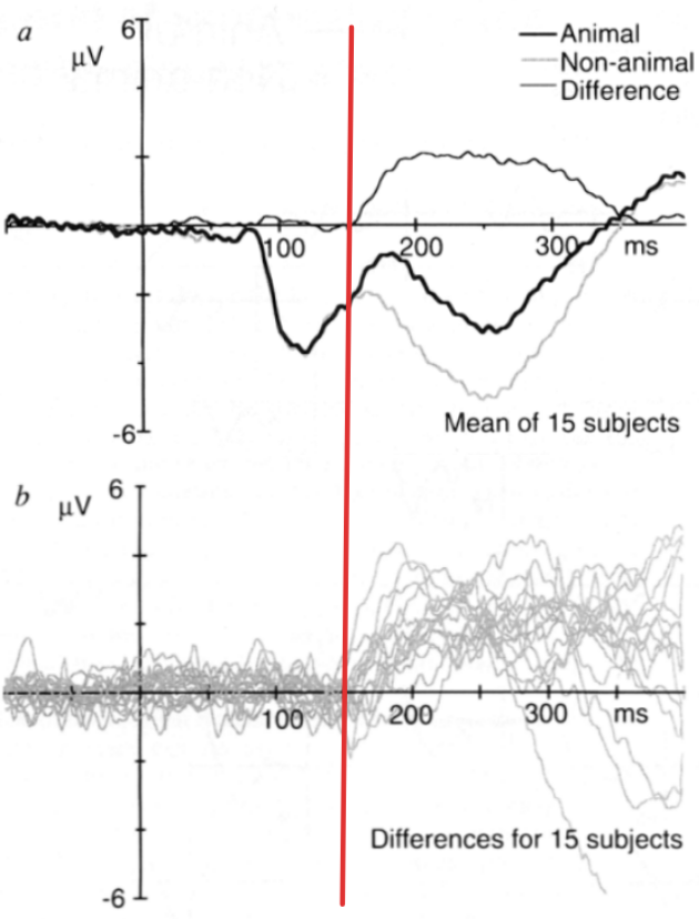
In 1996, Thorpe and colleagues used this RSVP paradigm in conjunction with electroencephalography, or EEG, which measures electrical activity in the brain with very high temporal resolution. They flashed images of animals and non-animals and asked subjects to perform a simple categorization task. What they found, as you can see on the plot, was outstanding. The EEG signal corresponds to the brain’s response to “animal” images, shown in darkest line, significantly diverged from the signal for “non-animal” images, shown in lightest line, at approximately 150 milliseconds after the image was presented. 150 milliseconds. To put that in perspective, a single blink of an eye takes about 300 to 400 milliseconds. This implies that the core computation underlying object recognition (from photons hitting the retina to a high-level semantic distinction) happens in a fraction of a blink. This is a critical insight that will strongly inform the design of the deep neural network we will talk about later.

And where in the brain is this happening? The advent of functional Magnetic Resonance Imaging, or fMRI, in the 1990s allowed researchers to start answering this question. While fMRI has poor temporal resolution, it has good spatial resolution, allowing us to see what brain regions are active during a task. Seminal work by Nancy Kanwisher and her colleagues called “The fusiform face area: a cortical region specialized for the perception of faces” identified specific regions in human brain that show preferential activation for specific high-level categories. For instance they discovered a region in the fusiform gyrus, which they termed the Fusiform Face Area or FFA, that responds quickly to faces than to other objects like houses. Conversely, they found another region, the Parahippocampal Place Area or PPA, that shows opposite preference: it responds strongly to scenes like houses, but not to faces. This provided concrete evidence for semantic organization and specialization within the higher level of the visual cortex.

So taking stock of these findings from neuroscience and cognitive science, a clear picture emerges. Visual recognition is a fundamental, core competency of visual intelligence. And the biological solution to this problem is incredibly fast, it exploited global context, and it appears to culminate in specialized representations for semantically meaningful categories. This understanding began to shift the focus of the computer vision community itself.

Toward face recognition (~1997–2001). Top row: output of segmentation methods (normalized‑cuts in 1997) showing region grouping into visually coherent “blobs”. Middle of timeline: SIFT (1999) introduces keypoint detection and robust local feature description based on invariant orientation and scale matching. Bottom-right: Viola–Jones face detection framework (2001) applies a cascade of Haar‑like feature classifiers to group evidence into fast, reliable face detections in real time

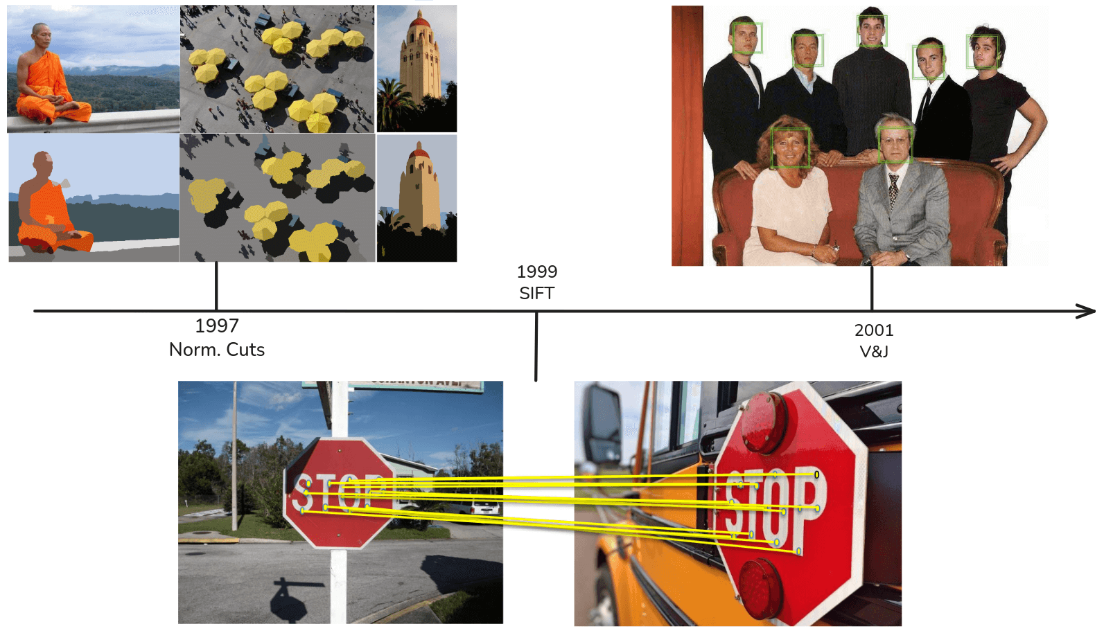
Coming out of the AI winter and into the 1990s, the field began to move away from pure edge detection and towards tackling the recognition problem more directly. One prominent approach was what we called “Recognition via Grouping”. The idea here is that a critical step towards recognition is to segment the image into perceptually meaningful regions. A landmark algorithm in this era was Normalized Cuts developed by Jianbo Shi and Jitendra Malik in 1997. As you can see, it takes an input image and groups pixels into coherent segments, effectively partitioning the image into a foreground object and a background. The underlying principle is based on graph theory, finding a cut in the pixel graph that minimizes a particular normalized cost. The thinking was, if we can achieve a good segmentation, recognition of the isolated object becomes a much simpler problem.

Then as we moved into the 2000s, another paradigm emerged that would become incredibly dominant: “Recognition via Matching”. The quintessential work here is David Lowe’s Scale-Invariant Feature Transform, or SIFT, from 1999. The core innovation of SIFT was a procedure to find a set of local, high distinctive keypoints in an image and to describe them in a way that is invariant to transformation like changes in scale, image rotation, and to some extent, illumination. Recognition then becomes a task of matching these keypoint descriptors between a query image, and a database of known objects. As you can see here, the algorithm can robustly find corresponding points to the stop sign, even though it’s viewed from a different angle and at a different scale. For about a decade, feature-based methods like SIFT were the state-of-the-art for many object recognition tasks.

And right at the turn of the millennium, in 2001, we see a truly landmark achievement that pointed to the future. This was the face detector developed by Paul Viola and Michael Jones. This was one of the first truly robust and real-time objective detections. It was so effective that it was quickly incorporated into consumer digital cameras, enabling the auto-focus-on-faces feature that we now take for granted. What was so revolutionary about the Viola-Jones detector was that it was one of the most highly successful applications of machine learning to a core computer vision problem. Instead of a human engineer meticulously designing feature to find faces, their algorithm learned a cascade of very simple rectangular features using a machine learning algorithm called AdaBoost, trained on a large dataset of positive examples (faces) and negative examples (non-faces). This was a critical turning point. It demonstrated, in a practical and impactful way, the power of a data-driven, learning-based approach over purely hand-engineered systems. And it’s this learning-based philosophy that, when taken to its extreme, will lead us to the deep learning revolution.

The rise, fall, and return of Neural Networks

So, we have now traced this timeline of computer vision up to the mid-2000s, We’ve seen the influence of neuroscience, the Marr paradigm, the focus on features like SIFT, and the nascent rise of machine learning. Now to understand what happens next, to understand the “deep learning” revolution we need to pause this timeline rewind all the way to the beginning, and pick up a completely different intellectual thread that was developing in parallel. This second thread also begins in the late 1950s, concurrent with Hubel and Wiesel’s discovery, in 1958, a psychologist named Frank Rosenblatt developed the Perceptron. The Perceptron was a simple computational model of a single biological neuron. It took a set of inputs, multiplied each by a corresponding weight, summed them up and if that sum exceeded a certain threshold it would output a “1”, otherwise “0”. It was simple, linear classifiers. And crucially, Rosenblatt devised a learning rule to automatically adjust the weights based on training examples.

However, this early enthusiasm for Perceptrons was dealt a severe blow in 1969 with the publication of the book Perceptron by Marvin Minsky and Seymour Papert. In this highly influential critique, they rigorously analyzed the mathematical properties of the single-layer Perceptron. They famously showed that there are certain, seemingly simple functions that a Perceptron is fundamentally incapable of learning. The canonical example is the logical XOR function.

The perceptron’s inability to solve XOR and its critique by Minsky & Papert.

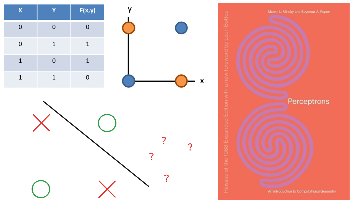
As you can see, the XOR function is true if one of its true inputs is true, but not both. If you plot the four possible input pairs, you find that you can not draw a single straight line to separate the ‘1’ outputs from ‘0’ outputs. Because the Perceptron is a linear classifier, it is mathematically impossible for it to solve this non-linearly problem. This critique was so powerful that it led to a significant decline in funding and research into neural networks, contributing to that first “AI winter” we discussed.

Despite this, some research continued, and in 1980, Kunihiko Fukushima in Japan developed a model called Neocognitron in a paper “Neocognitron: A Self-organizing Neural Network Model for a Mechanism of Pattern Recognition Unaffected by Shift in Position”. This is a truly remarkable piece of work, because it’s arguably the direct architectural ancestor of modern convolutional neural networks. The Neocognitron was explicitly and directly inspired by Hubel and Wiesel’s hierarchical of the visual cortex. It consisted of multiple layers, alternating between what Fukushima called S-cells and C-cells. The S-cells or simple cells, perform pattern matching using operations that are mathematically equivalent to what we now call convolution. The C-cells or complex cells, then provided spatial invariance by performing an operation analogous to what we now call pooling or subsampling. This is the fundamental architectural motif of a modern ConvNet. However, the Neocognitron had a critical limitation: it lacked a principled, end-to-end training algorithm. It was largely trained layer-by-layer with an unsupervised learning rule, and much of it was still hand-designed.

The missing piece of the puzzle arrived in 1986. In a landmark paper “Learning representations by back-propagating errors”, David Rumelhart, Geoffrey Hinton, and Ronald Williams popularized the backpropagation algorithm. Backpropagation is, in essence, an efficient method for computing the gradient of a loss function with respect to the weights of a multi-layered neural network. It’s a clever application of the chain rule from calculus. This algorithm provided the key that Minsky and Papert had pointed out was missing: a way to assign credit, or blame, to each neuron in each network, allowing one to systematically adjust the weights to improve performance. For the first time, it was possible to successfully train perceptrons with multiple layers, enabling them to learn non-linear function like XOR.

Top: Lenet, applied backprop algorithm to a Neocognitron-like architecture, learned to recognize handwritten digits. Bottom: Unsupervised pre-training technique by Hinton, Bengio, and others

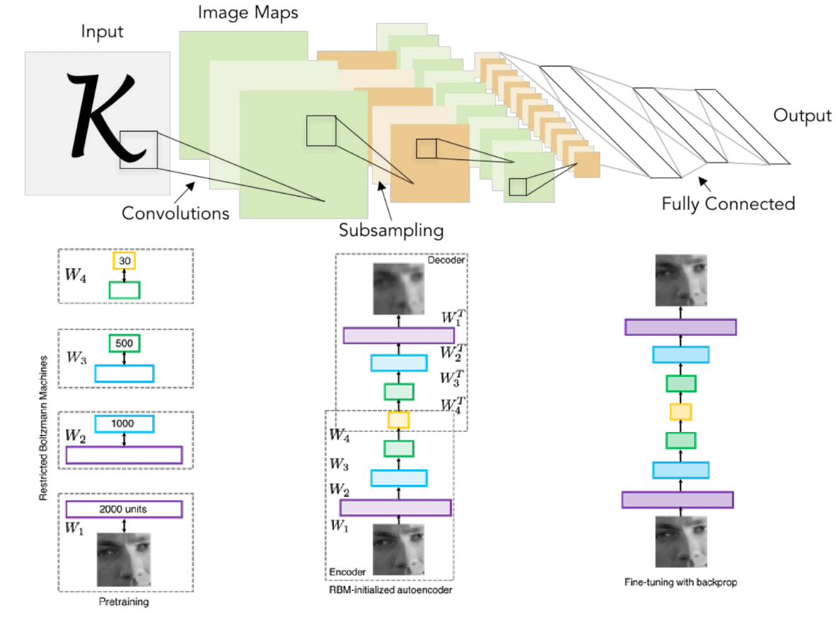
Now, we see the synthesis, in 1998, Yann LeCun and his colleagues took the Neocognitron architecture (with its alternating layers of convolution and pooling) and applied the backpropagation algorithm to train it from end-to-end on a real world task: recognizing handwritten digits. The resulting model, known as LeNet-5, was a tremendous success. It archived state-of-the-art performance and was deployed commercially by AT&T to read handwritten checks. If you look at this architecture diagram, it is strikingly similar to the convolutional neural networks we use today. This was a powerful proof of concept, demonstrating that these neurally-inspired, trained architectures could solve real, practical problems.

This success spurred a small dedicated community of researchers throughout the 2000s to explore what was then beginning to be called “Deep Learning”. The central idea was to build networks that deeper and deeper, with the hypothesis that more layers would allow the learning of more complex and hierarchical features. However, this was not yet a mainstream topic. Training these very deep networks proved to be extremely difficult due to the optimization challenges like the vanishing gradient problem. Researchers like Hinton, Bengio, and others developed clever techniques, like the unsupervised pre-training shown here, to try to initialize these deep networks in a better way before fine-tuning them with backpropagation.

The dataset that changed everything

Alright. So, the Viola-Jones face detector in 2001 gave us a powerful glimpse into the future, showing what was possible when you replaced hand-engineered rules with data-driven machine learning. This trend toward learning-based approaches and the need to rigorously evaluate them, led to another critical development in the field.

Left: The Caltech 101 images. Right: PASCAL Visual Object Challenge

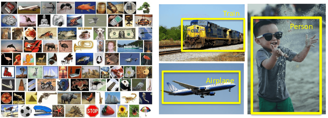
And that was the creation of standardized, large-scale benchmark datasets. Before the 2000s, it was common for researcher to test their algorithms on their own private, often small, collections of images. This made a direct, quantitative comparison of different methods exceptionally difficult. The establishment of datasets like Caltech101 in 2004, and later the PASCAL Visual Object Challenge, which ran from 2005 to 2012, was a major step in transforming computer vision into a more rigorous empirical science. PASCAL was particularly influential because it went beyond simple image classification. It challenged algorithms to perform more complex tasks like object detection drawing a bounding box around an object and semantic segmentation. These shared benchmarks created a common ground, a competitive arena, where the entire community could measure progress.

Still, deep learning remained something of a niche topic within a broader machine learning and computer vision community. And there was a fundamental reason for this. Even with these new algorithm tricks, these deep high-capacity models were incredibly data-hungry. They require vast amounts of labeled data to learn meaningful representations and to avoid overfitting. And in the mid-2000s, there was simply no good dataset to work on. The existing benchmarks, like Caltech101, were orders of magnitude too small to truly unlock the potential of these models. The algorithms were simply ahead of the data. And that brings us to the final, critical ingredient that would ignite the deep learning explosion. The ImageNet dataset.

ImageNet Large Scale Visual Recognition Challenge

Conceived and led by Fei-Fei Li, starting in 2007, the ImageNet project was an effort of unprecedented scale. The goal is to map out the entire noun hierarchy of WorldNet and populate it with millions of clean, annotated images. The result was a dataset with over 14 million images, spanning more than 20,000 categories. Crucially, in 2010, the project launched the ImageNet Large Scale Visual Recognition Challenge, or ILSVRC. This competition focused on a subset of the data: 1,000 object classes, with roughly 1.3 million training images. The task was straightforward: given an image, produce a list of five object labels, and you get credit if the correct label is in your list. This dataset and this annual challenge provide a perfect crucible. It was a dataset massive and complex enough to finally demonstrate the power of data-hungry deep learning models, and a competition that would pit them directly against the state-of-the-art classical computer vision system of the day. The stage was now set for a revolution.

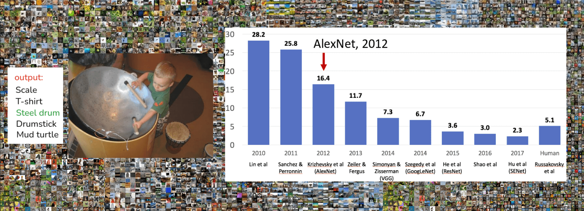
So, ImageNet sets the stage. Now let’s look at the performance on this challenge over the years. The bar chart above shows the top-5 error rate. That means the model gets five guesses, and if the correct label isn’t in those five, it’s an error. In 2010, the winning entry from Lin et al. had an error of 28.2%. In 2011, Sanchez & Perronnin improved this to 25.8%. These were typically system based on more traditional computer vision pipelines(hand-crafted features like SIFT or HoG), followed by machine learning classifiers like SVMs. Good progress, but still very high error rate. Then look at 2012. A massive drop to 16.4% with Krizhevsky et al.’s model, which we now famously know as AlexNet. We’ll talk a lot about AlexNet. The trend continues, 2013, Zeiler & Fergus: 11.7%, 2014, we see two big ones: VGG (Simonyan & Zisserman) at 7.3% and GoogLeNet (Szegedy et al.) at 6.7%. And then, a really significant milestone in 2015: ResNet (He et al.) achieved 3.6% error. Now, why is that 3.6% so significant? Look over the far right. Andrej Karpathy, when he was a PhD at Stanford and several others including Fei-Fei, did a study (Russakovsky et al. IJCV 2015) to benchmark human performance on the subset of ImageNet. And a well-trained human annotator gets around 5.1% top-5 error. So, by 2015, deep learning models were, for the first time, surpassing human-level performance on this specific, very challenging task! The progress didn’t stop there, 2016, 2017 saw even lower error rates with models like SENet

Now, let’s zero in on that pivotal moment, AlexNet, 2012. You see the red arrow pointing squarely at that 2012 bar. That 28% down to 16% was not an incremental improvement; it was a paradigm shift. This was the moment deep learning, specifically deep convolutional neural networks, truly announced its arrival and demonstrated its power to the broader computer vision community. AlexNet in 2012 right after Deep learning(2016) and ImageNet(2009), this isn’t a coincidence. The availability of a large dataset like ImageNet, coupled with the increasing computational power of GPUs, allowed deep learning models, which had been around conceptually for a while(you see LeNet from ’98, Neocognitron from ’80) , to finally be trained effectively at scale. AlexNet’s success fundamentally changed the direction of computer vision research. Almost overnight, people shifted from feature engineering to learning features directly from data using deep neural networks. And the rest, as they say, is history, as subsequent years on that chart. So, ImageNet provided the challenge, and AlexNet provided the breakthrough deep learning solution. The combination really superchanged the field, and it’s why we’re here talking about these powerful models.

A revolution in pixels

Okay, we’ve seen how AlexNet in 2012 was a watershed moment for deep learning in computer vision, dramatically improving performance on ImageNet. Now let’s look at what happened after 2012

Left: Publications at top Computer Vision conferences. Right: arXiv papers per month

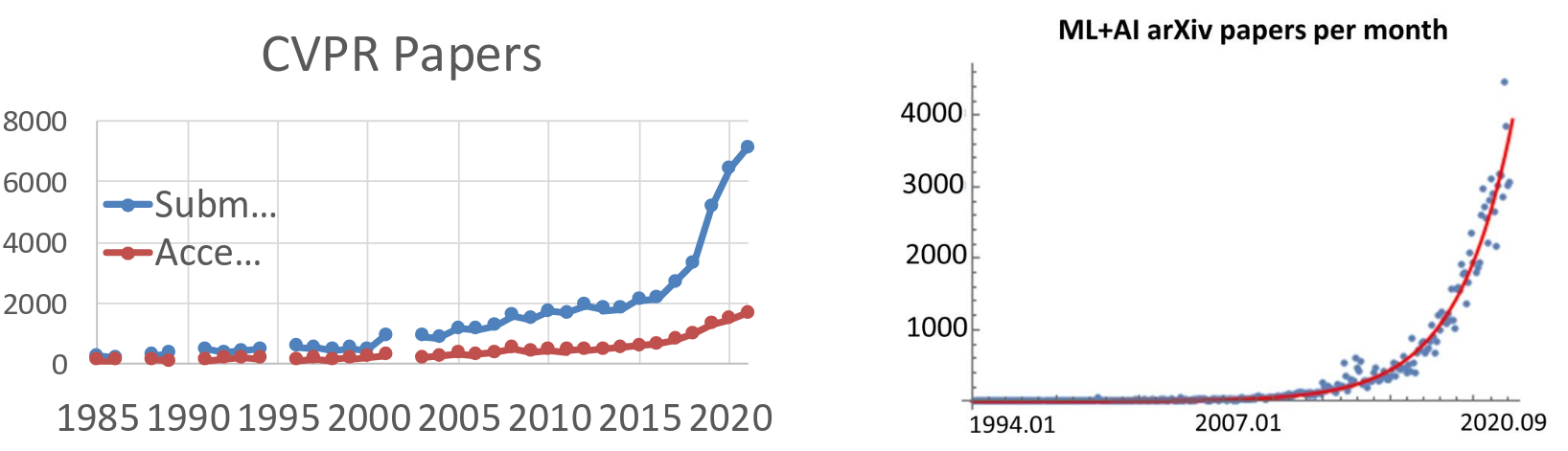
The graph on the left shows the number of paper submissions and acceptances to CVPR, which is one of the, if not the, top computer vision conferences. You can see a steady growth from 1985 up to around 2010-2012. But then, look what happens after 2012, especially the submissions. It just takes off, almost exponentially! We’re talking about going from around 2000, submissions to over 7000-8000 in just a few years. Now, the graph on the right shows the number of Machine Learning and AI papers uploaded to arXiv per month. arXiv, for those who don’t know, is a preprint server where researchers can upload their papers before or alongside peer review. This allows for very rapid dissemination of ideas. Again, we have a relative modest until around 2012-2013, and then it just skyrockets. We’re looking at thousands of ML/AI paper per month now. This isn’t just computer vision; it’s the broader AI field, but computer vision and deep learning are huge drivers of this trend.

So, we have an explosion of papers and research. But what kind of research? What were people working on? Let’s look at the winner of the ImageNet challenge each year following AlexNet:

• Year 2010(NEC-UIUC): Before the deep learning craze really hit ImageNet, this was what a state-of-the-art system looked like. You had a ‘Dense descriptor grid’ using features like HOG and LBP, then some ‘Coding’ (like local coordinate coding), ‘Pooling’ (Spatial Pyramid Matching - SPM), and finally a ‘Linear SVM’ for classification. This is a classic, handcrafted feature pipeline.
• Year 2012 (SuperVision, aka AlexNet): We’ve talked about this, Krizhevsky, Sutskever, and Hinton. It’s a stack of layers(convolutions, pooling, fully connected layers). This is a deep convolutional neural network, learning features directly from data.
• Year 2014 (GoogLeNet and VGG): Two years later, and we see even more sophisticated architectures.
  • GoogleNet (from Google, Szegedy et al.) the idea was to have filters of different sizes operating in parallel. It was also very deep but computationally quite efficient.
  • VGG (from Oxford, Simonyan & Zisserman) took a different approach: very simple, uniform architecture, just stacking 3x2 convolutions and 2x2 pooling layers deeper and deeper.
• Year 2015 (MSRA, aka ResNet): This was another huge leap, from Microsoft Research Asia(He et al.). This is ResNet, or Residual Network. They introduced ‘skip connections’ or ‘residual connections’ which allowed them to train networks that were incredibly deep, even over 100 or 1000 layers, which was previously impossible due to vanishing gradient problems. This architecture, or variants of it, became the backbone for many, many subsequent models.

So, in just a few years, we went from handcrafted pipelines to relatively shallow (by today’s standards) CNNs, to very deep and complex architectures, each pushing the boundaries of performance and what we thought was possible.

Now let’s look at what these models can actually do.

Deep learning is now everywhere

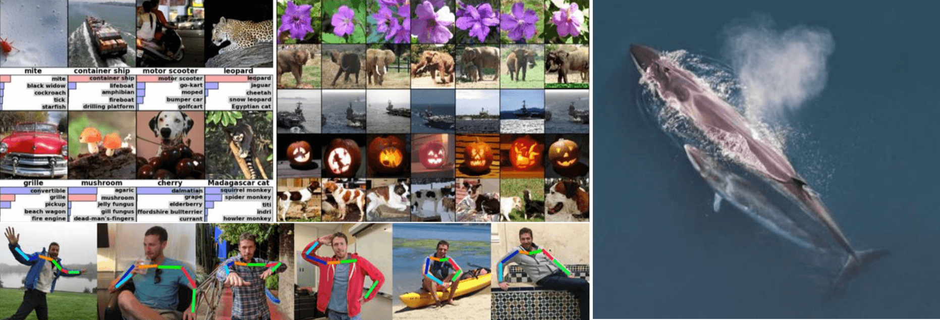
On the far left, we have examples of Image Classification from AlexNet back in 2012. For each image, the model outputs a list of probabilities for different classes, and here we see the top predictions. These aren’t just simple ‘cat’ or ‘dog’ classifications; the model is identifying specific types of objects, often in challenging, cluttered scenes. And these are real images, not just sanitized datasets. This was a clear demonstration of the power of these learned features. In the middle, we see an application called Image Retrieval. The idea here is: given a query image, can the system find visually and semantically similar images from a large database? These are just two fundamental computer vision tasks, classification and retrieval. But the success of deep learning, starting around 2012, has meant it’s now being applied to virtually every area of computer vision: object detection, segmentation, image captioning, image generation, video analysis, 3D reconstruction and so much more.

Continuing with the theme of understanding humans and dynamic scenes at the bottom, we have Pose Recognition also known as human pose estimation. The goal here is to identify the key joints of a person’s body like elbows, wrists, knees, ankles, head, shoulders. You can see in these examples (from Toshev and Szegedy, 2014, “DeepPose”, one of the first deep learning approaches for this) that the model can accurately locate these joints even with varied clothing, complex poses, and different backgrounds. This is fundamental for a deeper understanding of human actions, for animation, and augmented reality, and more.

And the reach of deep learning extends far beyond everyday scenes, videos, or games. It’s making significant impacts in highly specialized scientific and medical domains. On the far right, we have Whale Recognition. This might seem niche, but it’s important for ecological studies and conservation This particular image refers to a Kaggle challenge here is the link to the competition page, where participants build models to automatically identify individual whales from photograph. Deep learning is very good at these kinds of fine-grained visual recognition tasks

Top left: Image Captioning Vinyals et al, 2015 Karpathy and Fei-Fei, 2015. Top left: Krishna et al., ECCV 2016 the “Visual Genome” dataset and the work on generating scene graphs. Bottom: The Neural Style Transfer Algorithm (Gatys et al. 2016), which stylizes a photograph in the style of a given artwork

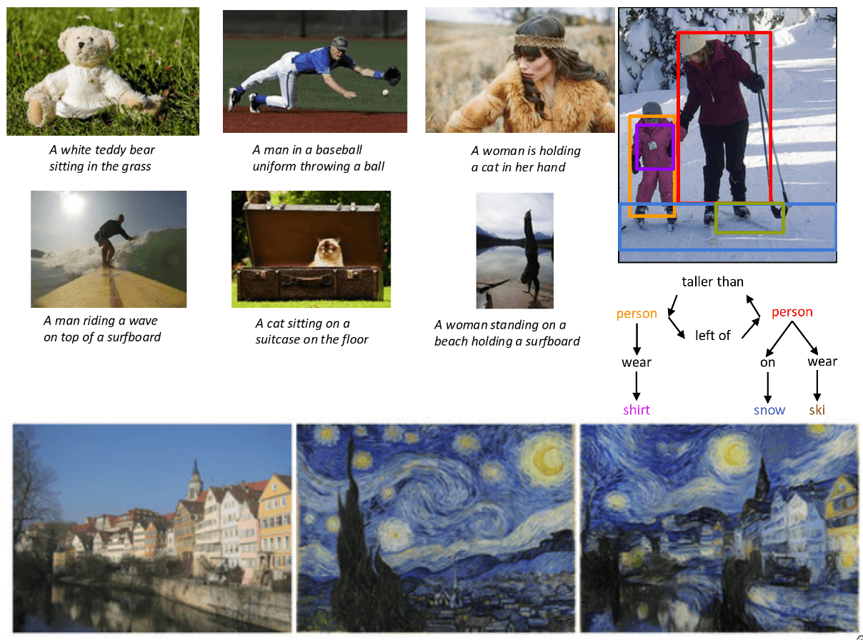
Now, this is where things get really interesting. We’re moving beyond just recognizing objects or pixels, and into the realm of understanding and describing images using natural language. This is Image Captioning. The task is, given an image, to automatically generate a human-like sentence that describes what’s happening in the image. These captions are remarkably accurate and fluent. This typically involves a combination of a Convolutional Neural Network (RNN), often an LSTM, to ‘generate’ the sentence word by word, conditioned on those visual features. The work here is from Vinyals et al. (from Google) and Karpathy and Fei-Fei (from Stanford), both published around 2015, were seminal works in this area, showing how to effectively combine CNNs and RNNs for this task. This was huge step toward machines that can not only see but also communicate what they see.

Image captioning gives us a sentence. But can we get a even deeper understanding of the relationships and interactions within an image? On the right you see an image with objects detected, and blow it we see something more structured: a scene graph. This moves us towards a much more comprehensive understanding of visual scenes. The work from Krishna et al. ECCV 2016, refers to the “Visual Genome” dataset and the work on generating a scene graph, which provides a dense, structured annotation of images, capturing objects, attributes, and relationships. This is crucial for tasks like visual question answering, where the model answers questions about an image and more complex reasoning about visual content.

So far, we’ve mostly seen deep learning used for understanding or analyzing images. But what about creating them? Or manipulating the artistic ways? At the bottom we see something called Neural Style Transfer pioneered by Gatys et al. in 2016. Here, you take two images, a content image here is the houses on the street and a style image like a famous painting like Van Gogh’s The Starry Night. The algorithm then synthesizes a new image that has the content of the first image but is rendered in the style of the second. So you get the houses looking as if they were painted by Van Gogh, or in a stained-glass style. This is done by optimizing an image to match content features from one image and style features (correlations between activations in different layers) from another, using a pre-trained CNN.

Continuing with generative models, we’ve shown artistic generation. But what about generating entirely new, photorealistic images from scratch? And this points to that capability, especially referencing Generative Adversarial Networks or GANs.

Sliced Wasserstein distance (SWD) between the generated and training images (Section 5) and multi-scale structural similarity (MS-SSIM) among the generated images for several training setups at 128 × 128. And (a-g) CELEBA examples corresponding to rows in Table 1. (h) the converged result

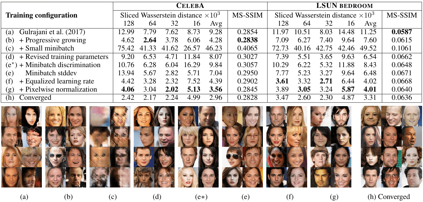
This is from Karras et al., for their work on “Progressive Growing of GANs for improved Quality” GANs, introduced by Ian Goodfellow and his colleagues in 2014, work by having two networks compete against each other. A Generator network tries to create realistic images for example from random noise. And a Discriminator network tried to distinguish between real images (from training set) and images created by the generator. Through this adversarial process, the generator gets better and better at creating images that can fool the discriminator, and the discriminator gets better at telling them apart. The “Progressive Growing of GANs” technique, developed by Karras and his team at NVIDIA was a major breakthrough. It allowed for the generation of much higher-resolution and more stable results than previously possible. They started by generating very small images like 4x4 pixels and then progressively added layers to both the generator and discriminator to produce larger and more detailed images like 8x8, 16x16, all the way up to 1024x1024. You can see from the image above, faces that are not real people, yet they look entirely plausible. This ability to synthesize photorealistic imagery has huge implications for art, design, entertainment, data augmentation, and of course, also raises important ethical considerations about ‘deepfakes’ and misinformation. But these generative capabilities truly underscore how far deep learning has come since 2012, from classifying images to creating entirely new visual realities.

We’ve seen some incredible generative capabilities, like GANs creating photorealistic faces. But what if we could guide that generation with more than just random noise or style images? What if we could tell the model exactly what we want it to create, using natural language?

Ramesh et al, “DALL·E: Creating Images from Text”, 2021, images from https://openai.com/blog/dall-e/

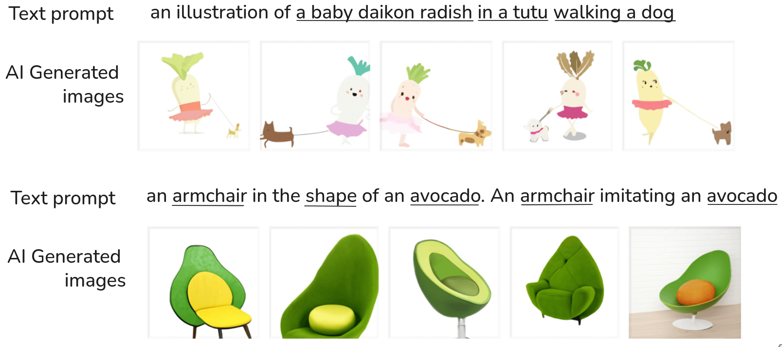
This brings us to one of the most mind-blowing developments in recent years: Text-to-image Generation. These are not images found on the internet these were created by an AI model based purely on that text description. And they are remarkably good! You see various interpretations, some look more like a cut avocado half turned into a chair, others are more abstract but clearly evoke both “armchair”and ‘avocado’. What’s so powerful about this (and models like DALL-E, Imagen, Stable Diffusion, etc.) is the compositionality and zero-shot generalization. The model has likely never seen an “armchair in the shape of an avocado” during its training. But it knows what armchairs are, it knows what avocados are, and it understands how to combine these concepts based on the textual relationships. The images above are from Ramesh et al, 2021, for DALL-E, a groundbreaking model from OpenAI. This kind of model is typically a very large transformer-based architecture, trained on massive datasets of image-text pairs. It learns to associate visual concepts with textual descriptions and can then generate novel images by combining these learned concepts in new ways. This ability to translate complex, even whimsical, textual prompts into coherent and creative visual outputs is a huge leap.

This isn’t just about fun images. It has profound implications for creative industries, design, content creation, and even help us understand how these large models represent and manipulate concepts. We’ve gone from classifying what’s in an image to generating entirely new visual realities from abstract textual descriptions. It’s truly an exciting time for AI and vision.

The spark and the fuel

So, we’ve spent a lot of time looking at this incredible explosion of deep learning applications from 2012 to the present. We’ve seen progress in classification, detection, segmentation, captioning, generation, and so much more. A natural question arises: Why now? What were the key ingredients that came together to make this revolution possible?

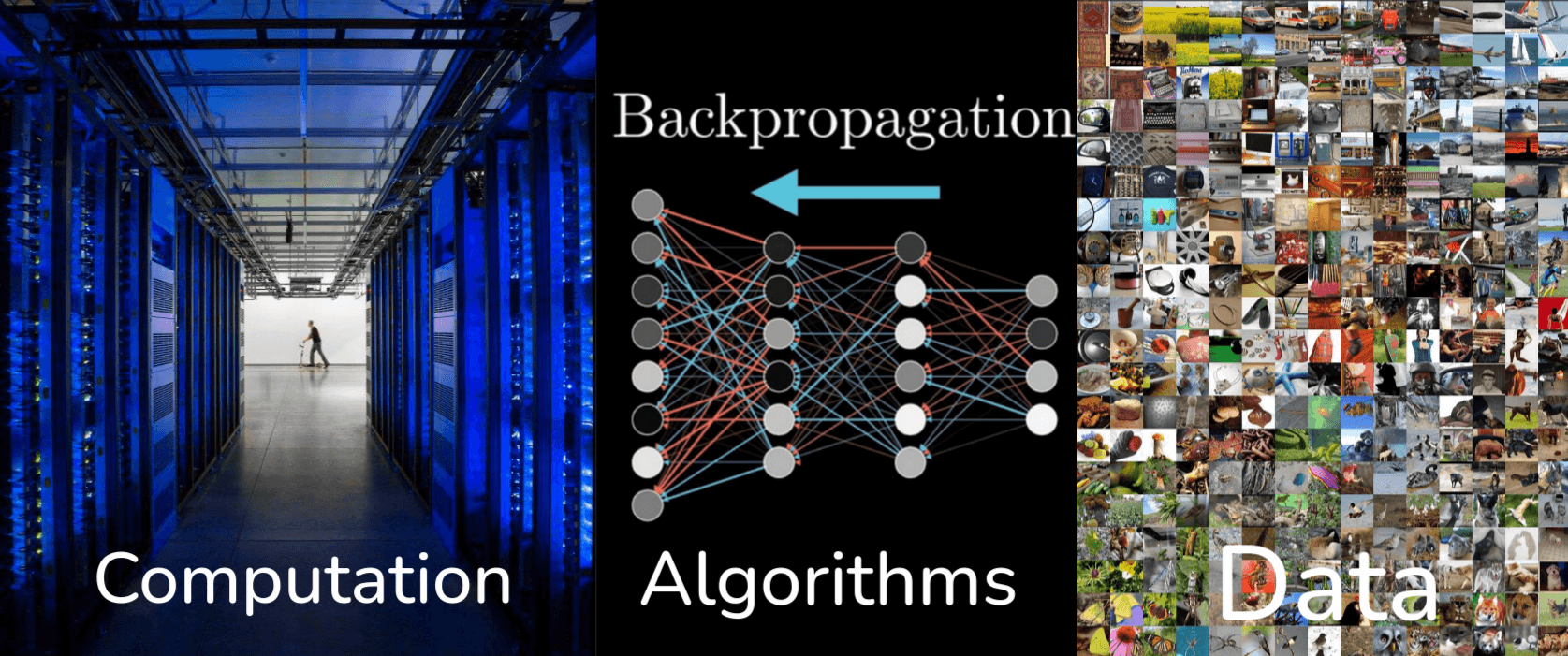
There are three main reasons. The Computation, Deep learning models, especially the large ones we’ve been discussing, are incredibly computationally intensive to train. They require billions or even trillions of calculations. The Algorithms, while many core ideas of neural networks have been around for decades, there have been significant algorithm innovations. These include new architectures like ResNet, Transformers, better optimization techniques, new activation functions, regularization methods, and so on, which have made it possible to train much deeper and more complex models effectively. And finally the Data, datasets like ImageNet, which we discussed, were crucial. Deep learning models are data-hungry, they learn by seeing millions of examples. The internet, social media, and large-scale data collection efforts have provided this fuel.

the GFLOP per Dollar graph. ‘GFLOP’ stands for Giga Floating Point Operations Per Second. It’s a measure of computational power (how many billions of calculations a processor can do in one second). The graph shows this metric per dollar, so it’s a measure of cost-effectiveness

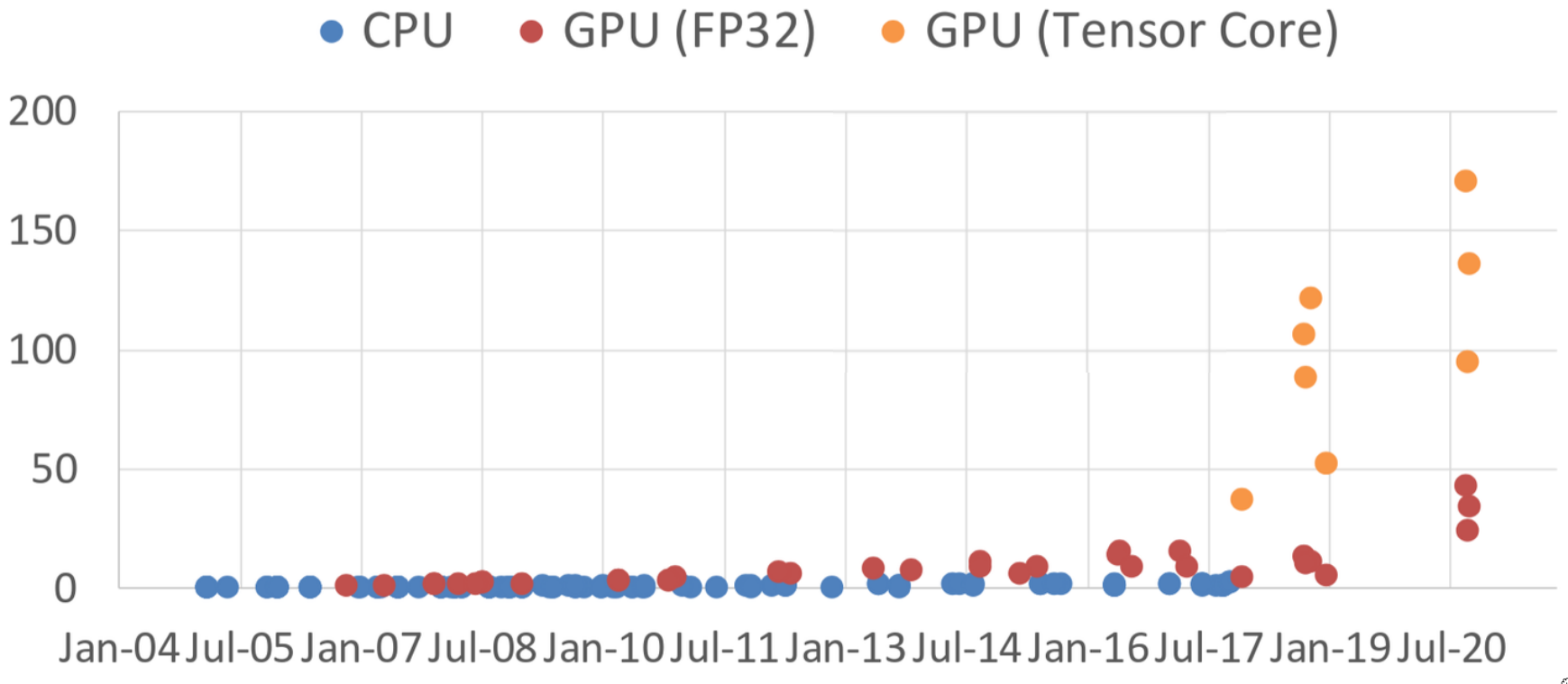
Let’s focus on the Computation aspect. Look at the dramatic difference between CPUs and GPUs starting around 2007-2008 with GPUs like the GeForce 8800 GTX which was one of the first to support general-purpose computing via CUDA. Around 2010-2012 we had GeForce GTX 580, this is the era when AlexNet was developed. Alex Krizhevsky trained AlexNet on NVIDIA GPUs, and their parallel processing capabilities were absolutely critical for training such a large network in a reasonable amount of time. Then we have the so-called “Deep learning Explosion” starting around 2012-2013, precisely when GPU performance and accessibility were taking off. Later GPUs like GTX 1080 Ti, RTX 2080 Ti, RTX 3090, and RTX 3080 continued this trend, offering massive parallel computation at increasingly better price points (or at least, significantly more power for a high-end card).

But the story doesn’t end there with the arrival of GPU (Tensor Core) which is a special hardware for deep learning. Starting with NVIDIA’s Volta architectures, GPUs began to include dedicated hardware nits specifically designed to accelerate the types of matrix multiplication and accumulation operations that are the heart of deep learning computations. These Tensor Cores can perform mixed-precision matrix math (e.g., multiplying FP16 matrices and accumulating in FP32) much, much faster than general-purpose FP32 units.

This is a fantastic example of a positive feedback loop:

1. Deep learning shows promise.
2. Researchers start using GPUs for their parallel processing capabilities.
3. The demand for deep learning computation grows.
4. Hardware manufacturers (like NVIDIA) see this massive market and start designing specialized hardware units like Tensor Cores to further accelerate deep learning workloads.
5. This new, even more powerful hardware enables researchers to train even larger, more complex models, pushing the boundaries of AI further.

So it’s not just that the GPU happened to be good for deep learning; the hardware itself has evolved because of deep learning, making it even more powerful and efficient for these tasks. This co-evolution of algorithms, software, and hardware is a key characteristic of the current AI boom.

Now let’s zoom out and look at the broader AI’s explosive growth and impact. This isn’t just an academic phenomenon, it’s having a massive real-world impact.

data = FileAttachment("./data/attendance-major-artificial-intelligence-conferences.csv").csv()

// Group data by conference
aaai_data = data.filter(d => d.Entity === "AAAI")
cvpr_data = data.filter(d => d.Entity === "CVPR")
iclr_data = data.filter(d => d.Entity === "ICLR")
icml_data = data.filter(d => d.Entity === "ICML")
neurips_data = data.filter(d => d.Entity === "NeurIPS")
total_data = data.filter(d => d.Entity === "Total")

// Create the Plotly chart
Plotly = require("plotly.js-dist@2")

chart = {
  const traces = [
    {
      x: aaai_data.map(d => d.Year),
      y: aaai_data.map(d => d["Number of attendees"]),
      type: 'scatter',
      mode: 'lines+markers',
      name: 'AAAI',
      line: { color: '#9467bd', width: 3 },
      marker: { size: 8 },
      hovertemplate: '%{fullData.name}: %{y:,}<extra></extra>'
    },
    {
      x: cvpr_data.map(d => d.Year),
      y: cvpr_data.map(d => d["Number of attendees"]),
      type: 'scatter',
      mode: 'lines+markers',
      name: 'CVPR',
      line: { color: '#1f77b4', width: 3 },
      marker: { size: 8 },
      hovertemplate: '%{fullData.name}: %{y:,}<extra></extra>'
    },
    {
      x: iclr_data.map(d => d.Year),
      y: iclr_data.map(d => d["Number of attendees"]),
      type: 'scatter',
      mode: 'lines+markers',
      name: 'ICLR',
      line: { color: '#ff7f0e', width: 3 },
      marker: { size: 8 },
      hovertemplate: '%{fullData.name}: %{y:,}<extra></extra>'
    },
    {
      x: icml_data.map(d => d.Year),
      y: icml_data.map(d => d["Number of attendees"]),
      type: 'scatter',
      mode: 'lines+markers',
      name: 'ICML',
      line: { color: '#8c564b', width: 3 },
      marker: { size: 8 },
      hovertemplate: '%{fullData.name}: %{y:,}<extra></extra>'
    },
    {
      x: neurips_data.map(d => d.Year),
      y: neurips_data.map(d => d["Number of attendees"]),
      type: 'scatter',
      mode: 'lines+markers',
      name: 'NeurIPS',
      line: { color: '#2ca02c', width: 3 },
      marker: { size: 8 },
      hovertemplate: '%{fullData.name}: %{y:,}<extra></extra>'
    },
    {
      x: total_data.map(d => d.Year),
      y: total_data.map(d => d["Number of attendees"]),
      type: 'scatter',
      mode: 'lines+markers',
      name: 'Total',
      line: { color: '#d62728', width: 3, dash: 'dash' },
      marker: { size: 8 },
      hovertemplate: '%{fullData.name}: %{y:,}<extra></extra>'
    }
  ];

  const layout = {
    title: {
      text: 'Conference Attendance Over Time',
      font: { size: 20 }
    },
    xaxis: {
      title: 'Year',
      showgrid: true,
      gridcolor: 'rgba(0,0,0,0.1)'
    },
    yaxis: {
      title: 'Number of Attendees',
      showgrid: true,
      gridcolor: 'rgba(0,0,0,0.1)',
      tickformat: ',d'
    },
    legend: {
      x: 0.02,
      y: 0.98,
      bgcolor: 'rgba(255,255,255,0.8)',
      bordercolor: 'rgba(0,0,0,0.2)',
      borderwidth: 1
    },
    hovermode: 'x unified',
    plot_bgcolor: 'white',
    paper_bgcolor: 'white',
    margin: { l: 80, r: 40, t: 80, b: 80 }
  };

  const config = {
    displayModeBar: true,
    displaylogo: false,
    modeBarButtonsToRemove: ['pan2d', 'lasso2d', 'select2d'],
    responsive: true
  };

  const div = DOM.element("div");
  div.style.width = "100%";
  div.style.height = "500px";

  Plotly.newPlot(div, traces, layout, config);

  return div;
}

This chart show the number of attendance at major AI conferences like CVPR(Computer Vision), NeurIPS(Neural Information Processing System, a top ML conference), ICML (International Conference on Machine Learning), AAAI (Association for the Advancement of Artificial Intelligence), ICLR (International conference on Learning Representations), and others, from around 2010 to 2024. Look at what happens around 2012-2015 onwards. The attendance for many of these conferences, especially those focused on machine learning and computer vision (like CVPR, NeurlPS, ICML, ICLR) just explodes. We’re talking about conferences going from a few thousand attendees to over 20,000, sometimes even more, in just a few years. This signifies a huge influx of researchers, students, and industry practitioners into the field. The source is from Our World in Data.

aiData = FileAttachment("./data/enterprise-ai-revenue.csv").csv()

aiChart = {
  const trace = {
    x: aiData.map(d => d.Year),
    y: aiData.map(d => d.Revenue),
    type: 'bar',
    name: 'AI Market Revenue',
    marker: {
      color: '#4285f4',
      opacity: 0.8,
      line: {
        color: '#1a73e8',
        width: 1
      }
    },
    text: aiData.map(d => `$${(+d.Revenue).toFixed(2)}`),
    textposition: 'outside',
    textfont: {
      color: '#333',
      size: 11
    },
    hovertemplate: '<b>%{x}</b><br>' +
                   'Revenue: $%{y:,.2f} million USD<br>' +
                   '<extra></extra>'
  };

  const layout = {
    title: {
      text: 'Enterprise Artificial Intelligence Market Revenue Worldwide 2016-2025',
      font: { size: 18 },
      x: 0.5
    },
    xaxis: {
      title: 'Year',
      showgrid: false,
      tickmode: 'array',
      tickvals: aiData.map(d => d.Year),
      ticktext: aiData.map(d => d.Year < 2025 ? `${d.Year}*` : `${d.Year}*`)
    },
    yaxis: {
      title: 'Revenue in million U.S. dollars',
      showgrid: true,
      gridcolor: 'rgba(0,0,0,0.1)',
      tickformat: ',.0f',
      range: [0, Math.max(...aiData.map(d => +d.Revenue)) * 1.1]
    },
    plot_bgcolor: 'white',
    paper_bgcolor: 'white',
    margin: { l: 80, r: 40, t: 100, b: 80 },
    showlegend: false
  };

  const config = {
    displayModeBar: true,
    displaylogo: false,
    modeBarButtonsToRemove: ['pan2d', 'lasso2d', 'select2d'],
    responsive: true
  };

  const div = DOM.element("div");
  div.style.width = "100%";
  div.style.height = "500px";

  Plotly.newPlot(div, [trace], layout, config);

  return div;
}

Next is Enterprise application AI revenue, the bar chart shows the revenue generated from enterprise applications of AI, in billions of U.S. dollars, from 2016 projected out to 2025. Even starting in 2016, there’s already noticeable revenue. But the projected growth is staggering. It goes from a few hundred billion dollars, and then projected to over thirty trillion dollars by 2025. This shows that AI is not just research or startups, it’s being deployed in established businesses across various sectors generating significant economic value. The source is from cloudlevante

Beyond the Benchmark

We’ve had a whirlwind tour through the incredible achievements of deep learning in computer vision since 2012. We’ve seen models classify, detect, segment, caption, and even generate incredibly realistic images. Now, it’s crucial to bring us back to reality and acknowledge that while the successes are profound, there’s still a lot of work to be done.

Despite the successes, computer vision still has a long way to go

We’ve achieved incredible feats on specific benchmarks, but true human-level visual intelligence, with common sense, robustness, and ethical considerations, is still a grand challenge. This isn’t to diminish the progress, but to inspire you for the future.

Source: https://www.washingtonpos t.com/technology/2019/ 10/22/ai-hiring-face-scan ning-algorithm-increasingly-decides-whether-you-deserve-job/ and https://www.hirevue.com/platform/ online-video-interviewing-software

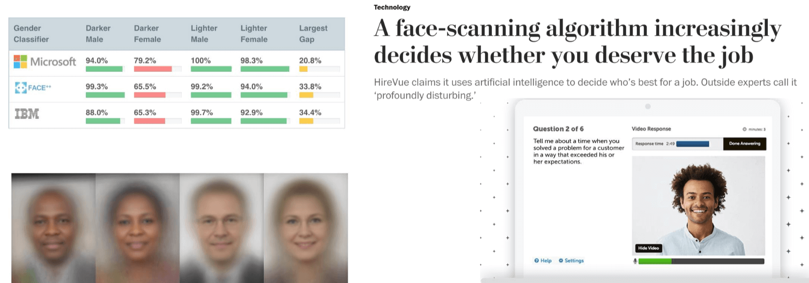
In fact, while computer vision can do immense good, it also has the potential to cause harm if not developed and deployed carefully. As future engineers and scientists in this field, it’s vital to be aware of those risks. Consider this concerned example Harmful Stereotypes, specifically related to gender classification. The table on the left shows the accuracy of gender classifiers from major tech companies like Microsoft, FACE++, IBM on different demographic groups. The largest gap column, while accuracy for lighter males and females is very high, it significantly drops for darker-skinned individuals, especially darker females. This means these systems are biased. Why does this happen? Often due to the lack of diverse and representative training data, or biases inherent in the data collection process. The averaged faces below visually represent these biased training sets. This is a critical issue, AI systems, if trained on biased data, will perpetuate and even amplify existing societal biases.

On the right, we see that can Affect people’s lives. The headline from The Washington Post: “A face-scanning algorithm increasingly decides whether”you deserve the job”. This refers to companies like HireVue, which use AI-powered video analysis in job interviews to assess candidates. The system analyzes facial expression, speech patterns, and other cues. While the intent might be to standardize hiring, outside experts call it “profoundly disturbing”. Imagine an algorithm, potentially biased, making decisions about your career prospects. This highlights that computer vision systems, when deployed in high-stakes environments like hiring, criminal justice, or healthcare, must be rigorously tested for fairness, transparency, and accuracy across all demographics. The ethical implications are enormous, and we, as a community, have a responsibility to address them.

But it’s not all about potential harm. We also need to recognize the immense potential for good. Computer vision can save lives. Consider the challenge of how to take care of seniors while keeping them safe? This is a growing societal problem with an aging global population. Computer vision offers a promising non-invasive solution. Imagine a camera system in a senior’s home, it can help early symptom detection of COVID-19 by monitoring cough, breathing changes, fever-like symptoms through thermal imaging. It can monitor patients with mild symptoms by reducing the need for frequent in-person visits. It can help manage chronic conditions like detecting changes in gait for mobility issues, monitoring sleep patterns, diet, or overall activity levels.

These systems are versatile and, crucially, scalable. They can be low-cost compared to continuous human care and can be burden-free for the seniors themselves, allowing them to maintain independence while providing peace of mind to their families and caregivers. This is a powerful example of how computer vision, when designed ethically and thoughtfully can be a force for immense societal benefit.

But even with these powerful applications, there are fundamental limitations in reasoning and common sense that remind us just how far we still have to go. This brings us to a classic, and still deeply relevant, thought experiment in computer vision.

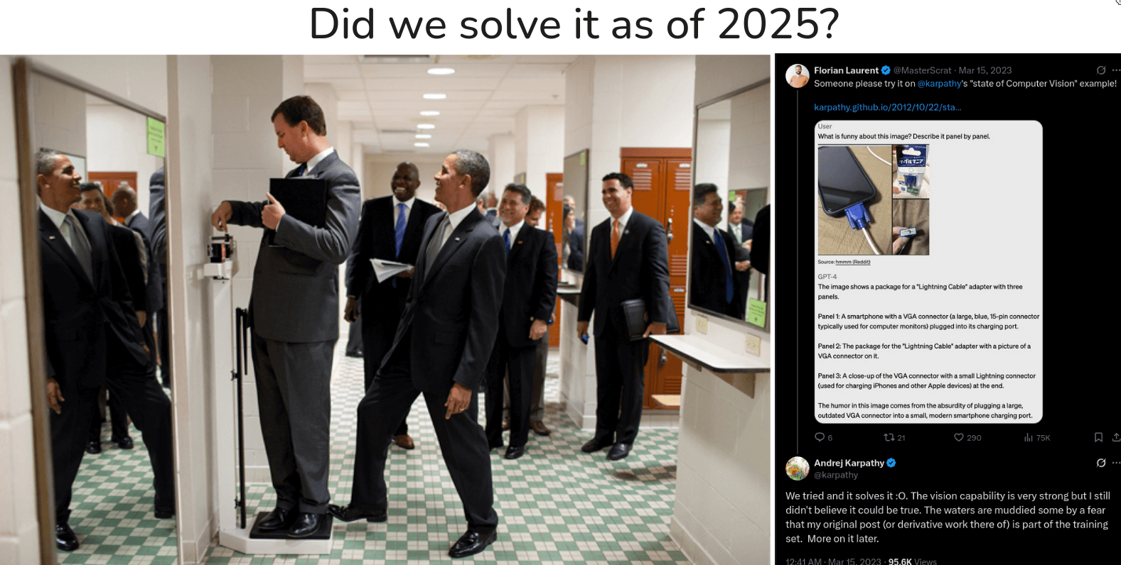
Back in 2012, Andrej Karpathy (who you may know as a former Director of AI at Tesla and a key figure in the field) wrote a blog post called “The state of Computer Vision and AI: we are really, really far away.” about the image you see above. He argued that it perfectly illustrated challenge facing AI. He called the state of computer vision at the time “pathetic” in the face of what this image requires. To truly understand the humor and the story in this photo, a computer would need to go far beyond just identifying pixels. It would need to synthesize an incredible amount of world knowledge.

First it needs to understand the complex scene geometry. It has to recognize people, but also realize that some of them are reflections in a mirror, not separate individuals.

Second it needs to grasp physical interaction and object affordance. It has to identify the object as a weight scale, understand that the person is standing on it to measure their weight, and then notice that then President Obama has his foot slyly placed on the back of the scale. This requires understanding that applying force to a scale alters its measurement a basic concept of physics.

But the real challenge, the part that truly tests intelligence, is reasoning about minds. The system would need to infer that the person on the scale is unaware of Obama’s prank because of his pose and limited field of view. It would need to anticipate the person’s imminent confusion when he sees the inflated number. Add it’s a deeply social, psychological, and physical understanding, all from a single 2D image of RGB pixels.

So, that was 2012. Now, let’s fast forward to the present day, over a decade into the deep learning revolution. Did we solve it? This very question resurfaced in 2023. When asked about the original Obama image, Karpathy’s response was telling:

We tried and it solves it :o.

For a moment, it seems like the problem was solved. But the story gets more complex. Karpathy immediately followed up with his own skepticism:

I still didn’t believe it could be true.

The reason for his doubt is a critical concept in modern AI: data contamination. The Obama photo is famous. It, along with Karpathy’s original blog post and thousands of articles explain the joke, and almost certainly part of the massive datasets used to train today’s large vision-language models. So, when the model “explains” the joke, is it truly reasoning from first principles, or is it performing an act of incredibly sophisticated retrieval? Is it recreating an explanation it has already seen, or is it generating one from scratch? Maybe the image might be leaked into the training set. This ambiguity is perfectly captured by Karpathy’s own words:

The waters are muddied…

And this is where we stand today, truly beyond the benchmark. The lines are blurring. Our models have become so powerful that we are no longer just asking “Is it accurate?” but the much harder question: “Does it understand?” The challenge is no longer simply about building a better classifier, but about building a system with verifiable reasoning, untangling true intelligence from phenomenal memory.

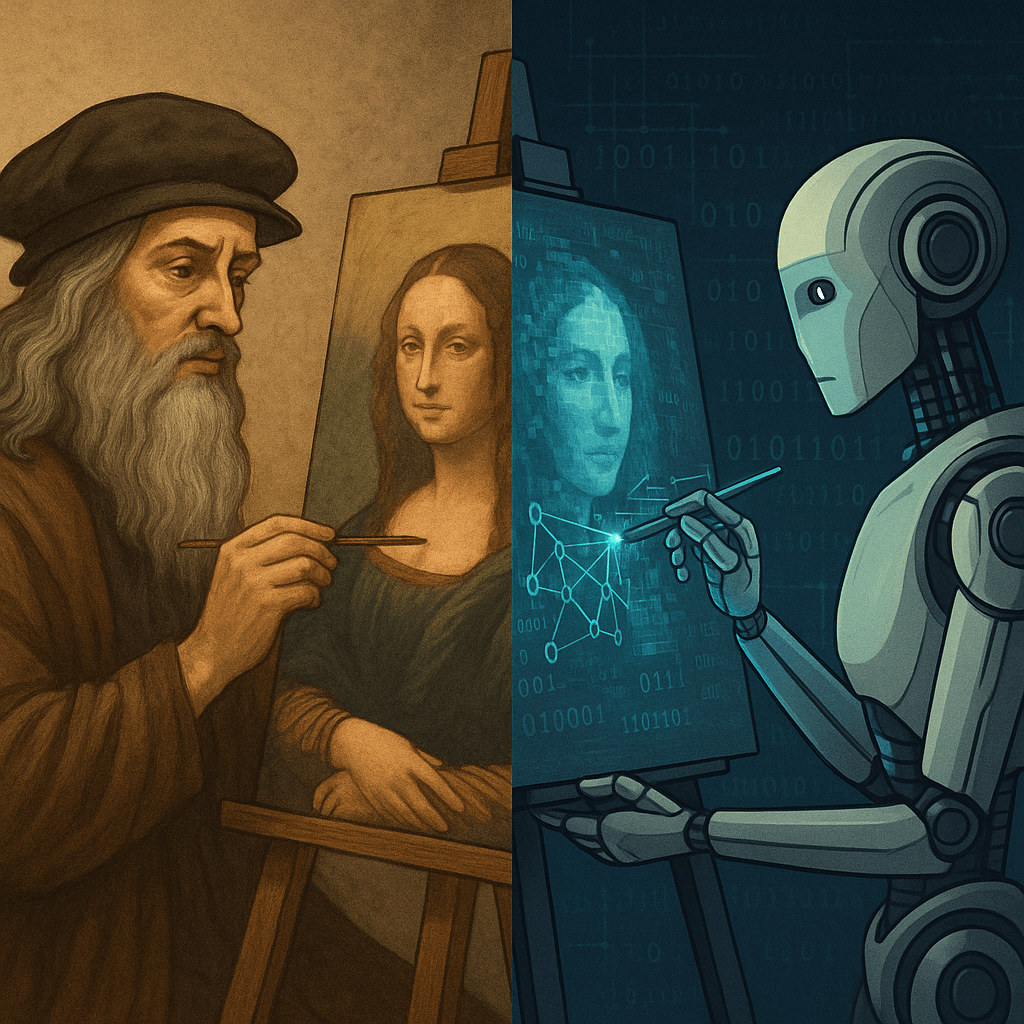
The road ahead is still long, but the problems we face are no longer just about recognizing pixels. They are about navigating ambiguity, context, and common sense which is the very fabric of intelligence itself. The canvas is far from finished, but the picture we are beginning to paint is more intricate and fascinating than we could have ever imagined.