Attentions and Transformers

Recurrent neural networks and the bottleneck

For the first time we step a way from static image and introduce this idea of Recurrent neural network, or RNN. These are really powerful and flexible class because they’re design to operate on sequential data.

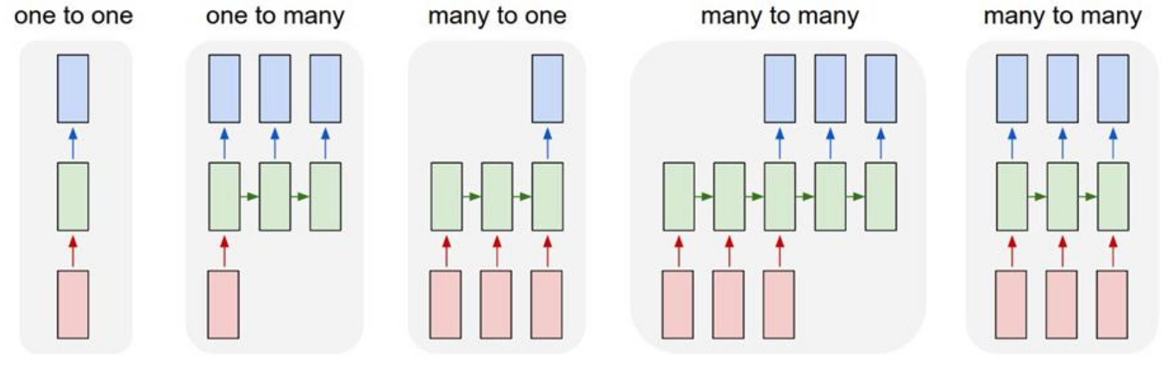
We see all these different architectures patterns: one-to-many for tasks like image captioning, many-to-one for something like video classification, and many-to-many for things like machine translation. The core idea is this recurrent connection - the hidden state that gets passed from one time step to the next, which gives the model a kind of memory. But these sequential processing and the way gradient flow time also introduces some pretty significant challenge especially dealing with very long sequences.

So, today, we’re going to build on that and introduce two new, very important concepts that address these challenges head-on: Attention and Transformers. First we’ll talk about attention, you can think of this as a new kind of building block, a new primitive operation for our neural network. At a high level, it’s a mechanism that operates on a set of vectors. It allow the model to dynamically focus on the most relevant part of the inputs when it’s producing an output. And that brings us to the Transformer. A transformer is a full-brown neural network architecture that uses this attention mechanism everywhere. It’s a very powerful design that completely get rid of sequential recurrence of RNNs and instead relies entirely on attention to model dependencies inputs and output.

Now, it’s really hard to overstate the impact that Transformers have had. They are everywhere today. They are the fundamental architecture behind the large language models you’ve heard about, like GPT and BERT, and more and more, they’re being applied to computer vision, often outperforming the convolutional networks that we’ve spent so much time on. But, before we can really understand the Transformer, I think it’s critical to understand where it came from. It didn’t just appear out of thin air. It actually developed as an offshoot of the RNN-based sequence-to-sequence models. The attention mechanism was first introduced to fix a fundamental bottleneck in those models. So, to properly motivate and understand why Transformers work the way they do, we need to go back to that starting point. So let’s start there

Alright, so to really understand where attention came from, let’s first dive deep into the problem it was designed to solve. And that problem arises in what are called sequence-to-sequence models built with RNNs

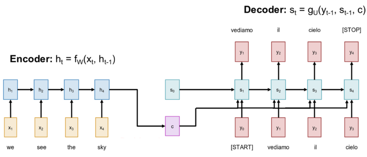
So let’s set up the problem. The task is “sequence-to-sequence.” We have an input sequence of vectors, x₁ through x_T, and we want to produce an output sequence, y₁ through y_T’, where the lengths T and T’ can be different. A great, motivating example for our whole discussion today is machine translation. Let’s say we want to translate a sentence from English to Italian. Our input sequence might be the words “we see the sky.” The standard way to tackle this with RNNs is with an architecture called an Encoder-Decoder.

\[ h_t = f_w(x_t, h_{t-1}) \]

The first part of this model is the Encoder. Its job is to read, or “encode,” the entire input sequence. So we take our first input word “we,” pass it into an RNN cell, and it produces a hidden state h1. Then, at the next time step, we take the next word “see” and the previous hidden state h1 to produce the new hidden state h2. And we just repeat this process for the entire input sequence, one word at a time, until we’ve processed the last word, “sky,” and produced our final hidden state h4. This is exactly the RNN behavior. So, once we’ve read the entire input sequence, what happens? Well, the whole idea here is that the final hidden state of the encoder, h_T (or h₄ in this case), has to somehow summarize the meaning of the entire input sentence. We take this final hidden state and we call it the context vector, which we will label c. This single vector c is the only piece of information that gets passed from the encoder to the next part of the model. It’s supposed to be a fixed-size summary of the entirely input. We also use this context vector to define the initial hidden state s₀, for the decoder

\[ s_t = g_U(y_{t-1}, s_{t-1}, c) \]

This brings us to the second half of the model, the Decoder. The decoder is another RNN, and its job is to take that context vector c and generate the output sequence, word by word. So how does it start? It’s initialized with hidden state s₀ that we got from context vector. To kick of the generation process, we feed a special [START] token as its first input, which we call y₀. The decoder RNN then process its state s₀ and the input y₀, and it produces two things: an output y₁, which is the first word of our translated sentence, “vediamo,” and a new hidden state, s₁. Notice that the context vector c is used as an input at every step of the decoder, constantly reminding it of the original sentence. Okay, so what happens at the next time step? This is where it gets interesting. The model operates in what’s called an “auto-regressive” fashion. That means the output from the previous step becomes the input for the current step. So, we take the word we just generated, “vediamo” (y₁), and feed that back into the decoder as the input for the next time step. The decoder then takes its previous state s₁ and this new input y₁ to produce the next state s₂ and the next output word, y₂, which in this case is “il.” And this process just continues. We feed “il” back in as input, the decoder produces “cielo.” We feed “cielo” back in as input, and eventually, the decoder will produce a special [STOP] token, which tells us that the sentence is complete and we can stop the generation process.

So just summarizing the whole flow: the encoder reads the input sequence and squashes it all down into one context vector. The decoder then text that context vector and unrolls it, generating input sequence one word at a time, feeding its own prediction back in as input.

Alright, so this architecture seems pretty reasonable, right? It was state-of-the-art for several years. But there’s a really fundamental problem with this design. And the problem is the input sequence bottlenecks through a fixed-size context vector c. Think about it. The entire meaning of the input sequence, all the word, their order, their grammatical relationships all of it has to be compressed and stuffed into this single vector. For a short sentence like “we see the sky,” maybe that’s plausible. But now, as a thought exercise, what if you’re translating a whole paragraph? What if your input sequence length T is 1000? You’re asking the model to summarize a thousand words of nuanced information into a single vector of maybe 512 or 1024 numbers. That is an immense information bottleneck. The model is almost certainly going to forget information, particularly from the beginning of the sequence. It puts a tremendous amount of pressure on the model to represent everything perfectly in this one vector.

The attention mechanism

So, what’s the solution? Well, what if we could remove this bottleneck entirely? The core idea, and this is really the key conceptual leap, is to allow the decoder to look back the whole input sequence at each time step of the output generation. Instead of relying on a single summary, at every time step where it’s trying to produce an output word, the decoder can have direct access to every single hidden state from encoder. This way it can dynamically decide which part of the input are most relevant to the specific word it’s about to generate. This is the central idea behind attention.

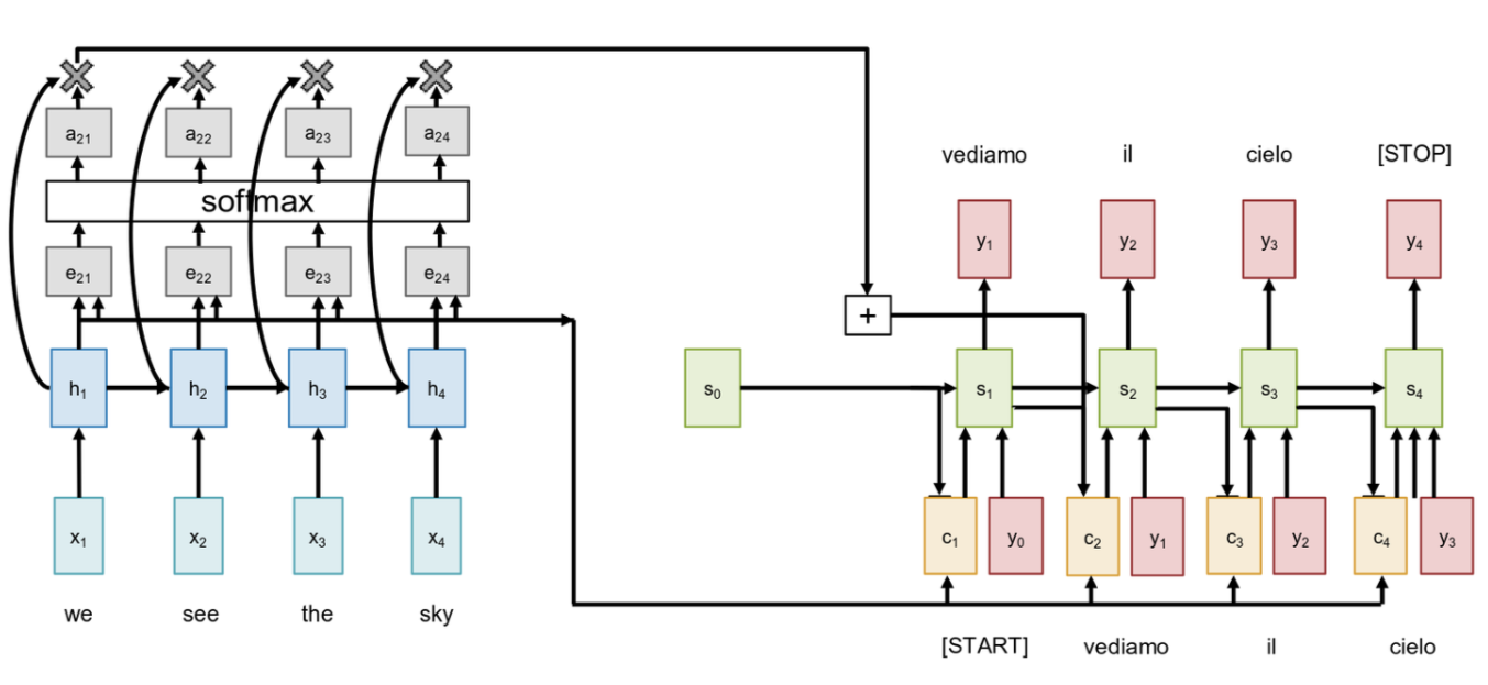
This is the Sequence to Sequence model with RNNs and Attention. This was first proposed in a paper “Neural Machine Translation by Jointly Learning to Align and Translate” by Bahdanau et al. in 2015, and it was a landmark result for machine translation. The encoder part of the model is exactly the same as before. We run an RNN over the input sequence, “we see the sky,” and we compute a hidden state h₁, h₂, h₃, h₄ for each input token. But here’s the crucial difference: we are no longer going to discard h₁, h₂, and h₃. We’re going to keep all of them. These encoder hidden states will be the values we “attend” to. We still use the final hidden state h₄ to initialize the decoder’s first hidden state, s₀, just to give it a starting point. So now we’re at the first step of the decoder. Our goal is to generate the first output word. To do this, we first need to figure out which of the input words are most relevant. We do this by computing a set of scale alignment scores. You’ll also see these called attention score. Let’s call them e_ti, which represent the score between the t-th decoder step and the i-th encoder hidden state. How do we compute this? We take our current state of our decoder and we compare it to each of the encoder hidden state, h₁ through h₄. This comparison is done by a simple neural network, f_att.

\[ e_{t,i} = f_{att}(s_{t-1}, h_i) \]

In practice, this is often just a simple linear layer, sometimes with a tanh activation function. It’s a trainable function that takes two vector, a decoder state and an encoder state and splits out a single scalar number that present how well they match or align. Now we have these raw alignment scores e. But they’re just arbitrary real numbers. What we want is a distribution. We want to know what proportion of our attention should go to each input word. So, the next step is to normalize these alignment scores to get attention weights, which we’ll call a. And the natural way to turn a set of arbitrary scores into a distribution is to use a softmax function. We apply a softmax over all the alignment scores for this time step. The resulting attention weights, a₁₁ through a₁₄, now have some nice properties: they are all between 0 and 1, and they all sum to 1. So they form a proper probability distribution over the input sequence.

Alright, so now we have these weights that tell us how much to focus on each input word. What do we do with them? The next step is to compute our context vector c_t, as a weighted sum of the encoder hidden states. So for our first time step, c₁ will be \(a_{11} \cdot h_1 + a_{12} \cdot h_2 + a_{13} \cdot h_3 + a_{14} \cdot h_4\). This is the most critical part of the whole mechanism. Instead of one static context vector for the whole decoding process, we are now computing a new, dynamic context vector at every single time step. This context vector, c_t, is tailored specifically for generating the t-th output word. It’s created by pooling information from the encoder states, weighted by how relevant they are for the current decoder state.

Now that we have this dynamically computed context vector c₁, the rest of the decoder step proceeds much like before. We feed this new context vector c₁ into our decoder RNN unit, along with the previous output y₀ (the [START] token). The RNN then updates its hidden state from s₀ to s₁ and predicts the first output word, y₁, which is “vediamo.” And the important thing to realize is that this whole process will repeat for the next step. To generate y₂, we will first use the new decoder state s₁ to re-calculate a whole new set of attention weights a_2i, which gives us a new context vector c₂, and so on. The context is no longer fixed, it’s recomputed for every single output token.

So let’s just pause for a second and build some intuition for what’s happening here. The context vector c_t now effectively attends to the relevant part of the input sequence. For our example, when we’re trying to generate the word “vediamo,” which corresponds to “we see,” it’s very likely that a well-trained model would learn to produce high attention weights a₁₁ and a₁₂ (for the inputs “we” and “see”) and low attention weights a₁₃ and a₁₄ (for “the” and “sky”). This means that the context vector c₁ would be composed mostly of the information from h₁ and h₂. It allows the model to focus its “attention” precisely where it’s needed. This completely resolves the bottleneck problem we identified earlier. Now a question you might have is: Where is the supervision for the attention weights come from? Do we need to separate the dataset to tell the model which input words a align with which output word? And the answer, which is really quite beautiful, is no. There is no direct supervision on the attention weights. The entire attention mechanism—the f_att linear layer, the softmax, the weighted sum is a fully differentiable computation. We can just plug it into our network, and we can backpropagate the final loss (from predicting the correct output word) all the way back through everything, including the attention mechanism. The model learns to produce sensible attention weights entirely on its own, through end to end training, simply because doing so helps it minimize the overall loss function. It’s a learned, latent alignment that emerge as a side effect of trying to solve the main task.

This new architecture is better in two critical ways. First, and most importantly, the input sequence is no longer bottlenecked through a single vector. We’ve completely remove that constraint. The decoder has direct access to the full sequence of encoder hidden state at every step. And second, following from that, at each timestep of the decoder, the context vector “looks at” different parts of the input sequence. As you can see in this simplified diagram, we compute a different context vector c₁, c₂, c₃ for each and every output step. This allows the model to create a soft, dynamic alignment between the source and target sequences, which is a much more powerful and flexible way to handle the relationship between them, especially for long and complex inputs. This idea of using attention to overcome the limitations of sequential processing was incredibly powerful. And it naturally leads to the next question: if attention is so good at relating different parts of a sequence, do we even need the recurrent part of the RNN at all? And that’s exactly the question that the Transformer paper set out to answer.

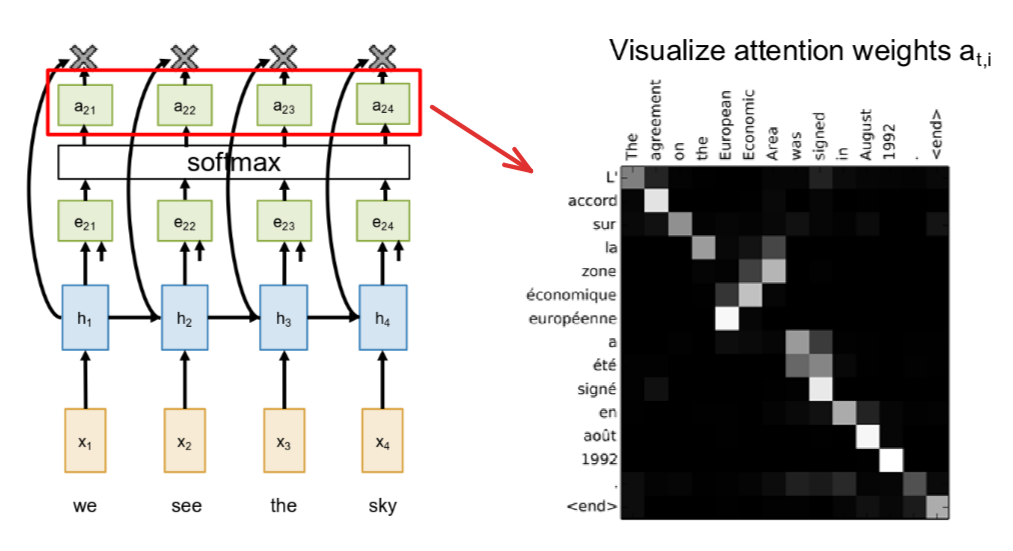
So here’s a famous visualization from that original Bahdanau attention paper. What they did was train an English-to-French translation model and then plotted the attention weights, a_ti, for a given sentence. What you’re looking at here is a matrix. The brightness of the pixel at position (i, j) tells you the strength of the attention weight. So, a bright pixel means that when the model was generating output word j, it was paying a lot of attention to input word i. Let’s look at the specific example here. The input sentence in English is: “The agreement on the European Economic Area was signed in August 1992.” And the model correctly translates this to the French output: “L’accord sur la zone économique européenne a été signé en août 1992.” Now, if you look at the structure of this attention map, you can see some really interesting patterns. For large parts of the sentence, the attention is strongly diagonal. You can see that when the model generates “L’accord,” it’s paying strong attention to “The agreement.” When it generates “sur la,” it’s looking at “on the.” Down at the end, when it generates “signé en août 1992,” it’s looking at “signed in August 1992.” This makes perfect sense because, for these parts of the sentence, the word order between English and French is pretty much the same. This diagonal alignment is a great sanity check; it shows us that the model has learned a very sensible, monotonic alignment between the two languages. But here’s where it gets really cool. Look at the part of the sentence that translates “European Economic Area.” In French, the word order is flipped: “zone économique européenne.” And look what the model does! The attention map is no longer diagonal here. When it generates the word “économique,” you can see a bright spot where it’s attending to the English word “Economic.” But then, when it generates the next word, “européenne,” it correctly looks back to the word “European” in the input. This is really powerful. It shows that the model isn’t just doing a simple, one-to-one mapping. The attention mechanism has allowed it to learn these non-trivial, non-monotonic alignments between the source and target languages. It figures out these complex word re-orderings all on its own, just through backpropagation.

Scaled dot-product attention

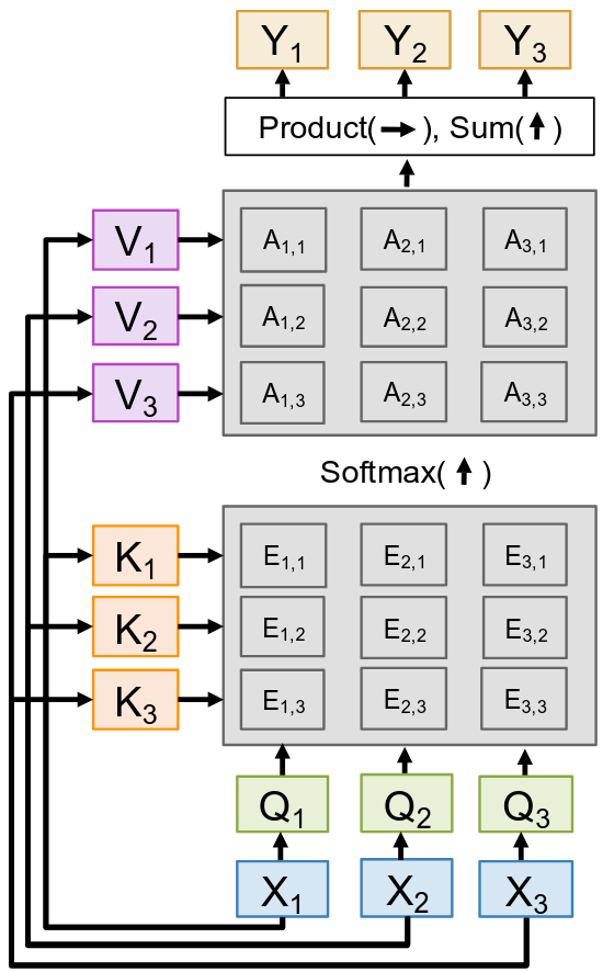
Let’s try to formalize this a bit using some new terminology. In this setup, we can think of having two sets of vectors. First, we have Query vectors. In our RNN example, these were the decoder hidden states (s₀, s₁, etc.). At each step, the decoder state is forming a query that essentially asks, “Given my current context, what information from the input is most relevant for me to generate the next word?” Second, we have data vectors, which are the encoder RNN states (h₁, h₂, etc.). These are the vectors that hold the information we want to retrieve. The query is posed against this set of data vectors. And the result of this operation is a set of output vectors, which in our case were the context vectors (c₁, c₂, etc.). So the core operation is this: Each query attends to all data vectors and give one output vector. That output vector is a summary of the data vectors, weighted by how relevant they are to that specific query. This Query-Data-Output framework is the general abstraction of the attention mechanism, and it’s the key idea that will let us move beyond RNNs entirely

So, let’s define the input for this layer. The first input is a single Query vector, which we’ll call q. This vector have some dimensionality, let’s say D_Q. . In our running RNN example, the query vector at the first time step was the initial decoder state, s₀. This is the vector that is “asking the question.”

The second input to our Attention Layer is a set of Data vectors, which we will represent as a matrix X. This matrix has N_X rows, where N_X is the number of data vectors, and D_X columns, for the dimensionality of each vector. In our RNN example, the data vectors were the set of N_X = 4 encoder hidden states, h₁ through h₄. These are the vectors containing the information that the query wants to selectively read from.

Okay, so those are the inputs: one query q and a set of data vectors X. Now let’s define the computation that happens inside the layer. The first step is to compute similarities. We take the query vector q and compare it to every one of the N_X data vectors X_i. This gives us N_X similarity scores, e_i, which we can collect into a vector e. Just like before, this similarity is calculated by some function f_att, which is typically a simple learned linear layer.

Step two: Once we have these raw similarity scores e, we need to normalize them into a distribution. So, we compute the attention weights, a, by simply applying a softmax function to the entire vector of similarity scores. The result, a, is a vector of length N_X where all the elements sum to 1. These weights tell us how much importance to assign to each of the data vectors.

The final step is to compute the single Output vector, which we’ll call y. This is done by taking a weighted sum of the data vectors X_i, using our just-computed attention weights a_i as the coefficients. So, \(y = \sum_i a_i \cdot X_i\). The dimensionality of this output vector y will be D_X, the same as the data vectors, because it’s just a linear combination of them. In our RNN example, this output vector was the context vector c₁. And that’s it! We have now defined a complete, self-contained Attention Layer. It’s a differentiable module that takes one query vector q and a set of data vectors X as input, and produces a single output vector y that is a summary of X from the perspective of q.

Now, let’s start refining this layer to get to the specific formulation that’s used in the Transformer model. We’ll make a few small but important changes. The first change is how we compute the similarity. In our general definition, we just said we use some function f_att, which is typically a small neural network. It turns out that in practice, we can do something much simpler and more efficient. We can just use the dot product between the query vector q and each data vector X_i. So the new similarity calculation is simply \(e_i = q \cdot X_i\). This is computationally very fast, and it works well. For this to be possible, of course, the dimensionality of the query D_Q and the data vectors D_X must be the same.

Okay, so that’s a nice simplification. But it turns out that if you just use a plain dot product, you can run into problems during training, especially when the dimension of these vectors is large. So this brings us to our second change: we don’t just use the dot product, we use a scaled dot product. We compute the dot product just as before, but then we scale it down by dividing by the square root of the dimension of the data vectors, \(\sqrt{ D_X }\). So the similarity is \(e_i = (q \cdot X_i) / \sqrt{ D_X }\). This might seem like a weird, magical detail, but it’s actually incredibly important for stabilizing the training process. So, let’s do a quick thought experiment to understand why this scaling is so critical. If we have very large similarity values, these will cause the softmax function to saturate, which in turn leads to vanishing gradients, making the model very hard to train. So, why would the dot product values become large? Well, let’s think about the dot product \(q \cdot X_i\). Suppose the components of q and X_i are independent random variables with zero mean and unit variance. Then the variance of their product is also 1. The dot product is a sum of D_X of these products. So, the variance of the dot product itself will be D_X. This means that as the dimensionality of our vectors D_X grows, the magnitude of our dot products will also grow. And if the inputs to a softmax function are very large in magnitude, the softmax output will be pushed to be very hard, one value will be very close to 1, and all the others will be very close to 0. When the softmax is in this saturated state, its gradients are extremely small, close to zero. And if the gradients are zero, no learning can happen. So, by dividing by \(\sqrt{ D_X }\), we are effectively normalizing the variance of the dot product back to 1. This keeps the inputs to the softmax in a reasonable range, prevents saturation, and allows gradients to flow properly during training. It’s a crucial trick for making these models work.

Alright, so we’ve refined our similarity calculation. The next generalization is to handle not just one query vector at a time, but a whole set of them. So instead of a single query vector q, our input will now be a matrix Q of shape [N_Q x D_X], containing N_Q different query vectors. And the beauty of using dot products is that this entire computation can now be expressed as a single, highly efficient matrix multiplication. To get all the similarity scores E, we just compute \(Q \cdot X^T / \sqrt{D_X}\). The softmax is applied to each row of this similarity matrix. And the final output Y is just the attention weight matrix A times the data matrix X. So now our Attention Layer takes a set of N_Q queries and a set of N_X data vectors, and it produces a set of N_Q output vectors. Each output vector Y_i is a weighted sum of the data vectors, where the weights are determined by the i-th query.

Inputs:

• Query vector: Q [N_Q x D_Q]
• Data vectors: X [N_X x D_X]
• Key matrix: W_K [D_X x D_Q]
• Value matrix: W_V [D_X x D_V]

Computation:

• Keys: \(K = XW_K\) [N_X x D_Q]
• Values: \(V = XW_V\) [N_X x D_V]
• Similarities: \(E = QK^T / \sqrt{𝐷_𝑄}\) [N_Q x N_X], \(E_{ij} = Q_iK_j / \sqrt{𝐷_𝑄}\)
• Attention weights: A = softmax(E, dim=1) [N_Q x N_X]
• Output vector: \(Y = AV\) [N_Q x D_V], \(Y_i = \sum_j A_{ij} V_j\)

Okay, one final change, and this will bring us to the complete formulation of what is called Scaled Dot-Product Attention, which is the core building block of the Transformer. We’re going to introduce a distinction between Keys and Values. The motivation here is that for each item in our input set, the vector we use to compute similarity (the “key”) might not be the same as the vector we use to compute the output (the “value”). This gives the model more flexibility. So what we do is we take our original data vectors X and we project them through two different learned linear layers, two weight matrices W_K and W_V, to produce a Key matrix K and a Value matrix V. Now, the computation proceeds like this:

1. The Queries Q are compared against the Keys K to compute the similarity scores.
2. We use these scores to get our attention weights A.
3. And finally, we use these attention weights A to take a weighted sum of the Values V.

Self-Attention

So, this entire operation that we’ve just visualized taking one set of vectors Q and another set X to produce an output Y has a name. This is called a Cross-Attention Layer. It’s called “cross-attention” because the queries are coming from one source, and the keys and values are coming from a different (or “cross”) source. Each query produces one output, and that output is a mixture of information from the data vectors, with the mixing proportions determined by the query’s similarity to the keys. This is precisely the type of attention we used in the sequence-to-sequence RNN model. The decoder states were the queries, and the encoder states were the source for the keys and values. Now, this naturally leads to a very interesting question: what happens if the queries, keys, and values all come from the same set of vectors?

This brings us to our next topic. What if the two sets of vectors were actually the same? What if a sequence wanted to attend to itself? This brings us to what is arguably the most important component of the Transformer: the Self-Attention Layer. So let’s define this. In a Self-Attention Layer, we only have one set of input vectors, X. There’s no separate set of queries. Instead, the Queries, Keys, and Values are all derived from this same input set X. This is the central idea. For each input vector X_i in our sequence, we are going to generate a query Q_i, a key K_i, and a value V_i by projecting X_i through three separate, learnable weight matrices: W_Q, W_K, and W_V. Because the queries and the keys/values now come from the same source, the shapes get a little simpler. The number of queries N_Q is now the same as the number of keys/values N_X, so all our matrices like E and A will be square: [N x N]. And in practice, we almost always set the dimensions of the queries, keys, and values to be the same, so D_Q = D_K = D_V. The core concept here is that each input produces one output, and that output is a mixture of information from all inputs in the sequence. It’s a mechanism for each token in a sentence to look at all the other tokens in that same sentence and build a new, more context-aware representation of itself.

Inputs:

• Data vectors: X [N x D_in]
• Key matrix: W_K [D_in x D_out]
• Value matrix: W_V [D_in x D_out]
• Query matrix: W_Q [D_in x D_out]

Computation:

• Query: \(Q = XW_Q\) [N x D_out]
• Keys: \(K = XW_K\) [N x D_out]
• Values: \(V = XW_V\) [N x D_out]
• Similarities: \(E = QK^T / \sqrt{𝐷_𝑄}\) [N x N], \(E_{ij} = Q_iK_j / \sqrt{𝐷_𝑄}\)
• Attention weights: A = softmax(E, dim=1) [N x N]
• Output vector: \(Y = AV\) [N x D_out], \(Y_i = \sum_j A_{ij} V_j\)

Now, just as a quick practical note. We said we generate Q, K, and V by passing our input X through three separate weight matrices. As an implementation optimization, these three linear projections are often fused into one larger operation. Instead of three separate matrix multiplies, you can concatenate the three weight matrices W_Q, W_K, and W_V into one big matrix. You then do a single, large matrix multiplication of X with this fused matrix. The result is a wider matrix that you can then just slice or split back into your Q, K, and V matrices. Why do this? Well, it turns out that modern hardware like GPUs are much more efficient at performing one large matrix multiplication than three smaller ones. It reduces overhead and better utilizes the parallel processing capabilities of the hardware. So while conceptually they are three separate operations, in code you will almost always see this fused implementation for performance reasons.

Let’s consider permuting the inputs. On the right, our original input order was X₁, X₂, X₃. Now, what happens if we feed the exact same vectors into the layer, but we just shuffle their order? Let’s say the new input order is X₃, X₁, X₂. What’s going to happen to the output? Well, let’s trace the computation. The first step is to compute the queries, keys, and values. Since each Q_i, K_i, V_i triplet is generated only from the corresponding input X_i, if we permute the inputs X, then the resulting sets of Q, K, and V vectors will contain the exact same vectors as before, just in that new permuted order. The set of queries is {Q₁, Q₂, Q₃}, and it will still be that same set, just shuffled. Okay, what about the next step, computing similarities? The similarity matrix E is computed by taking the dot product of every query with every key. For example, \(E_{1,1} = Q_1 \cdot K_1\). If we shuffle the inputs, the dot product between Q₁ and K₁ will be exactly the same, it will just appear in a different position in the new, shuffled similarity matrix. The set of all pairwise similarities is identical; it’s just that the rows and columns of the matrix have been permuted. Next, the attention weights. The attention weights A are computed by applying a softmax to the rows of the similarity matrix E.

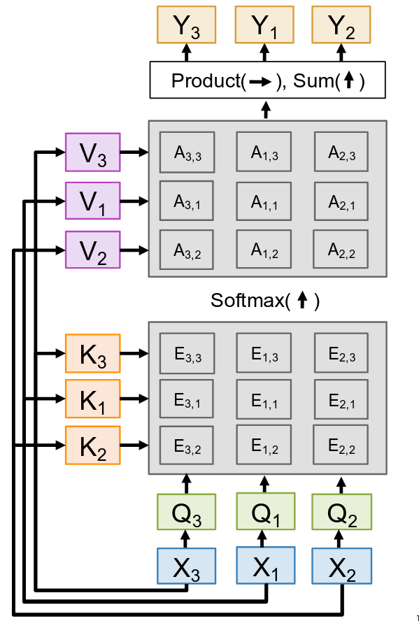
Since the values in E are just shuffled, the resulting attention weights A will also just be a permuted version of the original attention matrix. And finally, the outputs. Each output Y_i is a weighted sum of the value vectors. Since the value vectors V are the same set (just shuffled) and the attention weights A are also correspondingly shuffled, the final set of output vectors Y will be the exact same set of vectors we got before, just permuted in the same way as the original inputs.

So, what have we just demonstrated? We’ve shown that Self-Attention is permutation equivariant. This is a very important formal property. What it means is that if you have a function \(F\) (our self-attention layer) and you apply it to a permuted input \(\sigma(X)\), the result is the same as applying the function to the original input \(F(X)\) and then permuting the output in the same way \(\sigma(F(X))\). The critical takeaway here is that this means Self-Attention naturally works on sets of vectors. It doesn’t have any built-in notion of order or position. It treats the input as an unordered bag of vectors, interacts them all with each other, and produces an output bag of vectors. Now, this property is both a strength and a major weakness. It’s a strength because it’s a very general and flexible operator. But for many of the tasks we care about, like processing language, the order of the sequence is absolutely critical. “The dog bit the man” means something very different from “The man bit the dog.” So we have a problem: Self-Attention does not know the order of the sequence. If we just feed in word embeddings, it has no idea which word came first.

So how do we fix this? We need to explicitly give the model information about the position of each element in the sequence. We do this by adding a positional encoding to each input vector. This positional encoding is just another vector. The key idea is that this vector is not learned; it’s a fixed function of the index* of the token. So, for the first input X₁, we add a specific vector E(1). For the second input X₂, we add a different specific vector E(2), and so on. By adding these unique positional markers to each input, we’ve broken the permutation equivariance. The input X1 + E(1) is now fundamentally different from X2 + E(2), even if X1 and X2 were identical. This gives the model the information it needs to understand and leverage the sequential order of the input. And we’ll talk more about how these encodings are actually constructed later.

Okay, so this brings us to the next important variant of self-attention, which is critical for the decoder part of a Transformer. But now let’s think about another scenario. What happens when we want to use self-attention for a task where the model is generating a sequence, one element at a time, and it’s not supposed to know what’s coming next? This brings us to a crucial variant of this layer. This is the Masked Self-Attention Layer. The guiding principle here is simple: Don’t let vectors “look ahead” in the sequence.

Let’s think about why this is so important. Imagine you’re training a language model. The task is, given the first three words of a sentence, to predict the fourth word. If we used a standard self-attention layer, the representation for the third word would be computed by attending to all the words in the sentence, including the fourth word we’re trying to predict! The model would be cheating; it would have access to the answer. It would learn a trivial solution of just copying the answer, and it would be completely useless at test time when it actually has to generate a new word without knowing the future.

So, we need to enforce causality. We need to ensure that when we compute the output for position i, the model can only attend to inputs from positions 1 through i, and nothing further. How do we do this mechanically? The trick is very clever. It happens right after we compute the similarity matrix E, but before the softmax. We override the similarity scores for any connection that looks forward in time by setting them to negative infinity. Let’s look at the diagram. When we’re computing the output for position 2 (using Q₂), we want it to be able to look at position 1 and position 2, but not position 3. So, we would set the similarity score E_2,3 to negative infinity. When we compute the output for position 1, it should only be allowed to look at position 1. So we would set E_1,2 and E_1,3 to negative infinity.

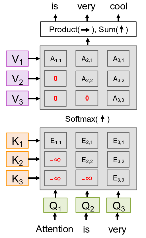
Now, why negative infinity? Think about the softmax function: e^x. What is e raised to the power of negative infinity? It’s zero. So, after we apply the softmax, all of these masked positions will have an attention weight of exactly zero. You can see this in the attention matrix A. The connections we wanted to forbid now have a weight of zero. This means that when we compute the final output vectors as a weighted sum of the value vectors, the model is physically incapable of pulling information from those future positions. We have effectively “masked out” the future. And as we’ve been discussing, this is absolutely critical for auto-regressive tasks like language modeling, where the goal is to predict the next word. If our input is “Attention is very,” and we’re trying to predict the next words (“cool,” “important,” etc.), the masked self-attention mechanism ensures that when we compute the output vector for “is,” it only uses information from “Attention” and “is.” When we compute the output for “very,” it only uses information from “Attention,” “is,” and “very.” This preserves the causal, step-by-step nature of generation that we need for these kinds of tasks. This masking is what allows a Transformer’s decoder to generate a sequence one token at a time, just like the RNN decoder did, but without the sequential bottleneck of an RNN.

Multi-head Self-Attention

So far, we’ve talked about self-attention as a mechanism where a sequence interacts with itself. We saw that a single self-attention layer learns to compute one specific kind of relationship between the tokens in a sequence, based on the dot-product similarity of their query-key pairs. But this raises a question. What if there are multiple different kinds of relationships we want to capture? For example, in a sentence, one token might relate to another syntactically (e.g., subject to verb), while also relating to a different token semantically (e.g., being a synonym). A single set of W_Q, W_K, and W_V matrices might struggle to learn all these different types of relationships at once. This is the motivation for our next idea. This is the Multi-headed Self-Attention Layer. The core idea is deceptively simple, instead of having one self-attention mechanism, we’re going to run H copies of self-attention in parallel.

We start with our same input vectors, X₁, X₂, X₃. But now, we’re going to have, in this example, H=3 independent self-attention layers. Each of these layers is called an “attention head.” And the critical part is that each head has its own, completely independent set of weights. So, head 1 has its own W_Q1, W_K1, W_V1. Head 2 has its own W_Q2, W_K2, W_V2, and so on. Because they have different weights, each head is free to learn a different kind of relationship. You can think of this as being very analogous to a convolutional layer in a CNN. A single convolution layer doesn’t have just one filter; it has many filters, and each filter learns to detect a different kind of visual feature (an edge, a color blob, a texture). Here, each attention head can learn to specialize in detecting a different kind of relationship within the sequence.

Okay, so we run our input X through these H parallel heads. What do we get? Well for each input token X_i, we now have H different output vector. As the diagram show, for input X₁, we now have an input from head 1 (Y_1,1), and output from head 2 (Y_1,2), and an output from head 3 (Y_1,3). So the next logical step is to gather these up. We can think of this as stacking or concatenating the independent outputs for each input position

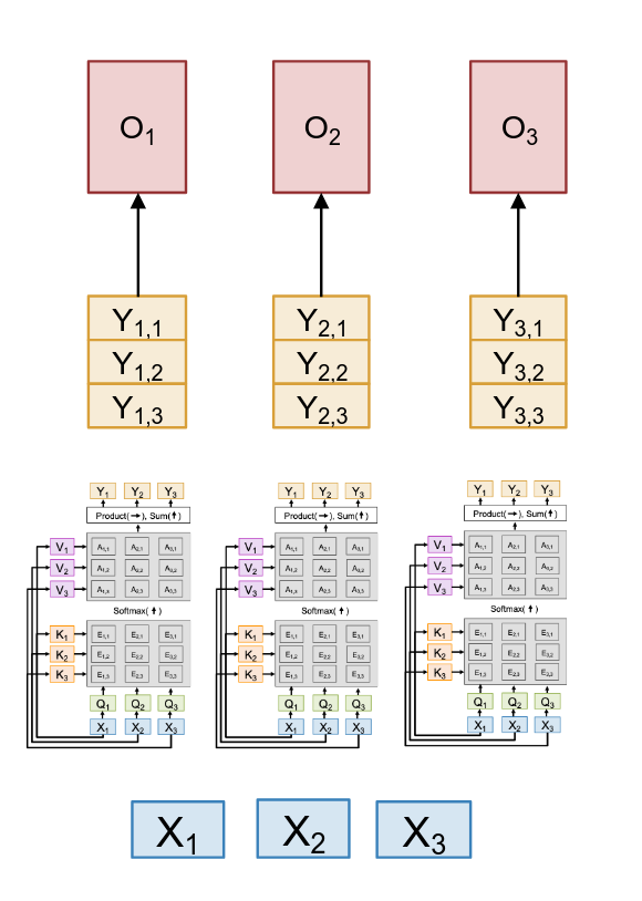
But we can’t just leave these outputs concatenated. We started with one vector per position, and we want to end up with one vector per position so we can feed it into the next layer of the network. So, the final step of the multi-head attention layer is an output projection. We take the concatenated outputs from all the heads and we pass them through one more learned linear layer, which has a weight matrix W_O. This final projection fuses the information learned by all the different heads back into a single output vector, O_i, for each position. This projection layer learns the best way to combine the different specialized representations from each head.

Conceptually, we’re running H full self-attention layers in parallel. But that sounds computationally expensive. Let’s say our main model has an input dimension of D. Instead of each of the H heads working with vectors of dimension D, we first split that dimension up. Each head will work with smaller vectors of dimension D_H, which we call the “head dimension.” Typically, we set D_H = D / H. So, we project our input X (dimension D) down into smaller Q, K, and V vectors (dimension D_H) for each head. Then we perform the scaled dot-product attention in parallel for all heads. Finally, we concatenate the H output vectors of size D_H back together, which gives us a vector of size H * D_H = D. Then we apply that final output projection W_O.

And in practice, all of this can be implemented incredibly efficiently. We don’t actually run H separate for-loops. Instead, we can reshape our Q, K, and V matrices to have an explicit “heads” dimension, and then we compute all H heads in a single pass using batched matrix multiply operations, which are highly optimized on GPUs. So the takeaway here is that multi-head attention isn’t just an optional add-on; it is the standard. It allows the model to simultaneously attend to information from different representation subspaces at different positions. This mechanism is used everywhere in practice and is fundamental to the power of the Transformer architecture.

Fundamentally, self-attention boils down to just four main learnable matrix multiplications. The first one is the QKV Projection. As we discussed, this is where we take our input X and project it into the queries, keys, and values for all heads. In practice, this is done with a single large matrix multiply from [N x D] to [N x 3HD_H], which we then split and reshape to get our Q, K, and V tensors. So that’s our first learnable multiplication.

\[ [N \times D] [D \times 3HD_H] \Rightarrow [N \times 3HD_H] \]

The second big computation is the QK Similarity. This is where we multiply the Q and K tensors to get our similarity matrix E. This is the core of the attention mechanism, where every token is compared against every other token.

\[ [H \times N \times D_H] [H \times D_H \times N] \Rightarrow [H \times N \times N] \]

Inputs:

• Data vectors: X [N x D]
• Key matrix: W_K [D x HD_H]
• Value matrix: W_V [D x HD_H]
• Query matrix: W_Q [D x HD_H]
• Ouput matrix: W_O [HD_H x D]

Computation:

• Query: \(Q = XW_Q\) [H x N x D_H]
• Keys: \(K = XW_K\) [H x N x D_H]
• Values: \(V = XW_V\) [H x N x D_H]
• Similarities: \(E = QK^T / \sqrt{𝐷_𝑄}\) [H xN x N]
• Attention weights: A = softmax(E, dim=2) [H x N x N]
• Head outputs: \(Y = AV\) [H x N x D_H]
• Outputs: \(O = YW_o\) [N X D]

The third major multiplication is the V-Weighting. After we compute the attention weights A via softmax, we multiply that attention matrix by the V tensor to produce the head outputs Y. This is where we actually aggregate the information from the value vectors based on our computed attention scores. And the fourth and final learnable matrix multiplication is the Output Projection. We take the concatenated head outputs and pass them through our final weight matrix W_O to produce the final output O of the layer.

\[ [H \times N \times N] [H \times N \times D_H] \Rightarrow [H \times N \times D_H] \]

And the fourth and final learnable matrix multiplication is the Output Projection. We take the concatenated head outputs and pass them through our final weight matrix W_O to produce the final output O of the layer.

\[ [N \times HD_H] [HD_H \times D] \Rightarrow [N \times D] \]

So there you have it. The entire, complex-looking multi-head self-attention layer is really just these four core matrix multiply stages, glued together with some reshapes and a softmax.

Now, analyzing the computation this way allows us to ask some very important practical questions. For example: How does the amount of compute scale as the number of vectors N (our sequence length) increases? Let’s look at the four steps. The QKV projection and the Output projection are linear in N. If you double the sequence length, you double the work for those. But look at steps 2 and 3. The QK Similarity step involves multiplying a [… x N x D_H] matrix by a [… x D_H x N] matrix, which results in a giant [… x N x N] attention matrix. The V-Weighting step multiplies that [… x N x N] matrix by the [… x N x D_H] value matrix. Both of these operations are dominated by that N x N interaction. This means that the computational cost of self-attention is O(N²), quadratic in the sequence length. If you double the length of your input sequence, you quadruple the amount of computation. This is the single biggest architectural bottleneck of the Transformer. RNNs, by comparison, are linear, O(N), in their computational cost.

Now let’s ask a related but different question: How does the memory usage of this layer scale with N? Where is the biggest tensor we have to store in memory to do the computation and backpropagation? Again, the answer comes from looking at that intermediate attention matrix A. This is an [H x N x N] tensor. To compute the gradients during backpropagation, we need to have stored this matrix in GPU memory. And its size is also O(N²). This quadratic memory cost is an even bigger problem in practice than the compute cost. Let’s put some numbers on it. Suppose you’re working with a long sequence, say N=100,000 tokens. Maybe it’s a long document, or a high-resolution image treated as a sequence of patches. And let’s say you have H=64 heads. That H x N x N attention matrix would require 1.192 Terabytes of memory. That’s not a typo. Your standard high-end GPU might have 40 or 80 gigabytes of memory. You can’t even come close to fitting this matrix. This quadratic memory scaling is what has historically limited Transformers to relatively short sequence lengths, often just 512 or a few thousand tokens.

Now, I have to mention that this is a very active area of research, and there have been some incredible breakthroughs recently. An algorithm called FlashAttention, which came out in 2022, is a great example. The key insight of FlashAttention is that you don’t actually need to write out the full N x N attention matrix to memory. By being very clever about the order of operations and how data is moved between the different levels of GPU memory (SRAM and HBM), it’s possible to compute the exact same output without ever instantiating that giant matrix. It computes the output in small blocks, fusing the softmax and the V-weighting steps together. This reduces the memory requirement from O(N²) down to O(N). This single algorithmic improvement has been transformative, allowing Transformers to be trained on much, much longer sequences than were possible before. It’s a beautiful example of how deep algorithmic understanding of hardware can unlock new capabilities for our models.

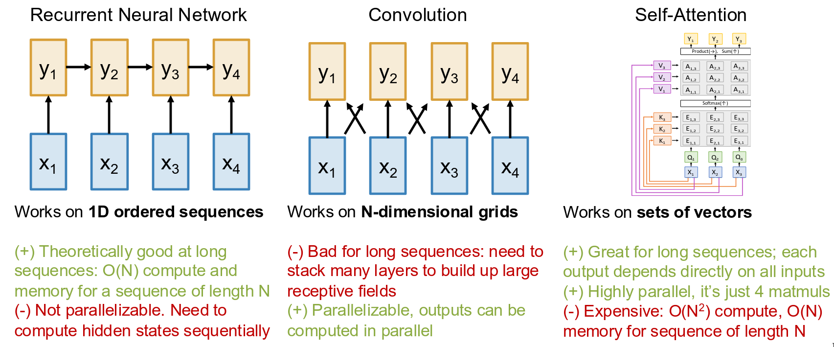
So if you look at this table, you see this fascinating set of trade-offs between these three fundamental operations. RNNs are slow but have an efficient O(N) scaling. Convolutions are fast but struggle with long-range dependencies. Self-attention is fast and directly models long-range dependencies, but has this expensive O(N²) scaling. And it was precisely by analyzing these trade-offs that the authors of the original Transformer paper made their big claim. They recognized the massive parallelization benefit of self-attention and saw that the long-range modeling was superior to convolutions. And they made a bet that they could build an entire architecture using only this self-attention mechanism, completely getting rid of recurrence and convolution. And this led to the landmark 2017 paper, famously titled: “Attention is All You Need.”. And with that, we are finally ready to put all of these pieces together and look at the full Transformer architecture.

The Transformer

The core building block of the entire Transformer architecture is what’s called a Transformer Block. So let’s build one of these blocks up, step by step.

Transformer block

The input to a Transformer block is a set of vectors x. Let’s say we have N=4 input vectors. Remember, because of what we learned about permutation equivariance, these also need to have positional encodings added to them, but we’ll leave that detail aside for the moment and just focus on the architecture of the block itself. Okay, so the very first thing we do inside a Transformer block is the operation we just spent all this time on. We pass the entire set of vectors through a (multi-headed) Self-Attention layer. This is the communication part of the block. This is where every vector x_i gets to look at every other vector x_j in the input set and produce a new, updated representation of itself that incorporates context from the entire sequence. Now, if you remember back to our CNN architecture, what was one of the most important innovations that allowed us to build really deep networks? It was residual connections.

And the Transformer architecture uses them everywhere. So, after the self-attention layer, we add a residual connection. We take the original input vectors x and add them to the output of the self-attention layer. This “add” operation is done element-wise for each corresponding vector in the sequence. Just like in ResNets, this helps with gradient flow and makes it possible to train very deep stacks of these Transformer blocks. The next component in the block is Layer Normalization. We used Batch Normalization to stabilize training. Layer Normalization is another type of normalization that serves a similar purpose. But there’s a key difference. Batch Norm normalizes across the batch dimension for each feature. Layer Norm, on the other hand, normalizes across the feature dimension for each individual data point in the batch. So for each vector coming out of our residual connection, we compute the mean and standard deviation of its elements and use them to normalize that vector. This was found to work much better than Batch Norm for sequence models like the Transformer. So, we apply a Layer Normalization step after the residual connection.

Okay, so we’ve had the communication part of the block (self-attention). Now we need the computation part. After the first Layer Norm, we pass each vector in the sequence independently through a small Multi-Layer Perceptron, or MLP. This is also sometimes called a Feed-Forward Network or FFN in the Transformer literature. It’s typically a simple two-layer MLP. You have a linear layer that expands the dimension (e.g., from D to 4D), followed by a ReLU activation, and then another linear layer that projects it back down from 4D to D. The important thing here is that while the self-attention layer mixes information across the sequence, this MLP operates on each position separately. It’s a per-position computation that adds more expressive power and allows the model to do more complex processing on the features at each location.

And what do you think comes after the MLP? You guessed it. Another residual connection. We take the input to the MLP block which was the output of the first layer norm and we add it to the output of the MLP. Again, this is crucial for building deep models. And finally, to finish off our Transformer block, we apply one more Layer Normalization step after that second residual connection. This produces the final output vectors y₁ through y₄ of our block.

So, this block takes a set of vectors x as input and produces a set of vectors y as output, with the same number of vectors. And it does this using two main computational motifs. First, there’s the interaction step. The only place in this entire block where information is mixed between different vectors in the sequence is inside that multi-head self-attention layer. That is the sole communication hub. Second, there’s the per-position processing. The LayerNorm and the MLP components all work on each vector independently. They process each position in the sequence in parallel, without any interaction between them. And as we’ve discussed, the whole thing is highly scalable and parallelizable. If you count them up, the vast majority of the floating point operations in this block are contained in just six matrix multiplications: the four from the multi-head self-attention layer (the QKV projection, the QK similarity, the V-weighting, and the output projection), and the two from the two-layer MLP. And as we know, matrix multiplications are something that modern hardware is incredibly good at.

So, what is a Transformer? It is really just a stack of these identical Transformer blocks. You take the output from the first block and feed it directly as the input to the second block, and so on. And what’s really remarkable is that this fundamental block architecture has not changed much since it was introduced in 2017. All of the massive models you hear about today are, at their core, just stacks of this exact same block. What has changed is that they have gotten a lot, a lot bigger. Let’s look at the scaling trend just to appreciate the numbers. The original Transformer from the “Attention is All You Need” paper, often called the “base” model, had 12 of these blocks stacked up. The model dimension D was 1024, it used 16 heads, and it was trained on sequences of length N=512. This model had about 213 million parameters. Which, at the time, was a very large model. But then things started to escalate quickly. Just two years later, in 2019, OpenAI released GPT-2. This was essentially just a larger version of the decoder part of the original Transformer. It had 48 blocks, a larger dimension of 1600, more heads, and could handle longer sequences of 1024 tokens. And this scaled the parameter count up to 1.5 billion. This was one of the first models that really captured public attention with its impressive text generation abilities. And the scaling just continued. The next year, OpenAI released GPT-3. Now we’re talking about 96 blocks, a massive model dimension of over 12,000, and 96 attention heads. This model clocked in at 175 billion parameters. And of course, the models we see today have continued this trend, pushing into the trillions of parameters. The key takeaway here is that this basic Transformer block has proven to be an incredibly scalable architecture. It seems that just by making these models bigger, more layers, larger dimensions, more heads and training them on more and more data, their capabilities continue to improve. This scaling law has been one of the most powerful and driving forces in all of AI over the last several years.

Transformer for language and vision

Now let’s get concrete and see how we would use this architecture to build a Large Language Model, or LLM, like GPT. The first thing we need to do is get our input into the right format.

Our Transformer blocks operate on sets of vectors, but our input is text-a sequence of words or tokens. So, the very first layer of the model needs to convert these words into vectors. We do this with a learnable embedding matrix. If our vocabulary has V unique tokens and our model’s hidden dimension is D, then this is simply a lookup table of shape [V x D]. For each word in our input sequence, like “Attention,” “is,” “all,” “you,” we look up its corresponding D-dimensional vector in this table. These embedding vectors are initialized randomly and are learned just like all the other weights in the network through backpropagation. This gives us our initial set of input vectors to feed into the first Transformer block. And of course, we would also add our positional encodings to these vectors at this stage.

Now, we feed this set of vectors through our stack of Transformer blocks. But there’s a critical detail we need to remember for language modeling. The task is to predict the next word in the sequence. This means the model must be causal; it cannot be allowed to look ahead. So, as we discussed earlier, we must use masked attention inside each of the self-attention layers in our Transformer blocks. This ensures that when the model is computing the output for token i, it can only attend to tokens 1 through i and is explicitly prevented from seeing any future tokens. Every self-attention layer in a model like GPT is a masked multi-head self-attention layer.

What we get out is a final set of contextualized output vectors, one for each input position.

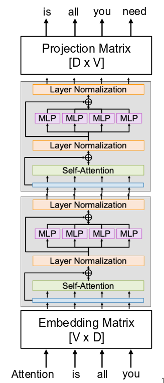
Now we need to make a prediction. For each output vector, we want to predict what the next word in the sequence should be. To do this, we need to go from our D-dimensional representation space back to the vocabulary space. So, at the very end of the model, we add a final projection matrix. This is a linear layer with weights of shape [D x V]. It takes each D-dimensional output vector from the last Transformer block and projects it into a V-dimensional vector. We can interpret this V-dimensional vector as a set of raw scores, or logits, for every single word in our vocabulary. The final step is to turn these scores into probabilities and compute a loss. For each position i, we take the V-dimensional logit vector and pass it through a softmax function. This gives us a probability distribution over the entire vocabulary, representing the model’s prediction for the word at position i+1. We can then compare this predicted distribution to the actual next word in the training data using a standard cross-entropy loss. We compute this loss for every position in the sequence and average them together. That final loss signal is then backpropagated all the way through the entire stack of Transformer blocks and the embedding matrix to update all the weights.

Okay, so this has been all about language. So, the natural next question is, can we use these same ideas for images? For a while, it seemed like CNNs were the undisputed kings of vision, and Transformers were for language. But then, in 2021, a paper “An Image is Worth 16x16 Words: Transformers for Image Recognition at Scale” came out of Google that completely changed that landscape. And that brings us to the Vision Transformer, or ViT.

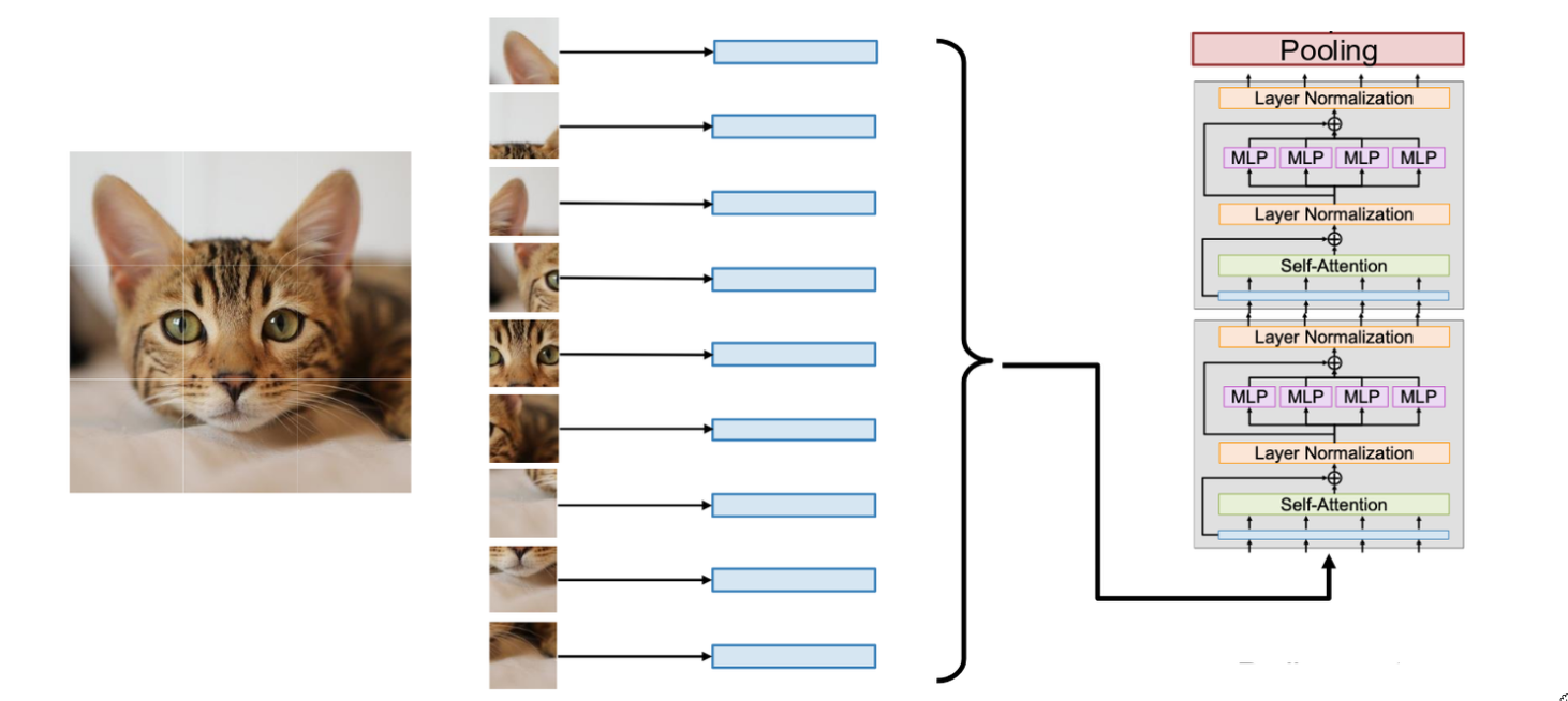
The core question the ViT paper asked was: can we apply a standard Transformer directly to an image for a task like image classification? The challenge is that a Transformer expects a sequence of vectors as input. But an image isn’t a sequence; it’s a 2D grid of pixels. For a standard 224x224 image, if you treated every single pixel as a token, you’d have over 50,000 tokens. And given the O(N²) scaling of self-attention, that would be computationally infeasible. So we need a different way to turn an image into a sequence.

The solution they proposed was remarkably simple and effective. Instead of treating pixels as tokens, they decided to break the image into a grid of non-overlapping patches. For example, you can take a 224x224 image and break it down into a grid of 16x16 patches. For a 224x224 image and 16x16 patches, this gives us a 14x14 grid, for a total of 196 patches. Each patch is 16x16x3 pixels. The next step is to turn each of these patches into a vector. So we take each patch, flatten its pixels into one long vector (16 * 16 * 3 = 768), and then apply a linear transformation to project it into our desired model dimension, D. This gives us what the Transformer wants: a sequence of N vectors, where N is the number of patches. Now let me pause here and ask a question. This whole operation of breaking an image into patches, flattening each patch, and then applying a linear projection… does that sound familiar? Is there another way we could describe this exact same operation using concepts we already know? This whole “patchify and project” operation is mathematically equivalent to taking the original image and running it through a single convolutional layer. Specifically, it’s a convolution with a kernel size of 16x16 and a stride of 16. The stride of 16 ensures that the filter is applied to non-overlapping patches. The kernel size of 16 ensures it sees the whole patch. The number of input channels is 3 (for RGB), and the number of output channels would be D, our model dimension. So, you can think of the ViT’s input processing as just a very large-stride convolution. It’s a nice way to connect this new architecture back to concepts we’re already very familiar with.

So now we have our sequence of N patch embedding vectors. What do we do with them? We just feed them directly into a standard Transformer encoder, which is just a stack of our Transformer blocks that we’ve already defined. These D-dimensional vectors for each patch are the input x to our stack of Transformer blocks. But wait, we’ve forgotten a crucial detail. Self-attention is permutation equivariant. It doesn’t know where each patch came from. The patch from the top-left corner is treated the same as the patch from the bottom-right. So, just like with language, we need to add positional encodings. In ViT, these are learnable vectors that are added to the patch embeddings. There’s a unique positional encoding for each possible patch position (e.g., for each spot on the 14x14 grid), which tells the model the original 2D position of each patch.

Now, what kind of attention should we use? Should it be masked? For image classification, the answer is no. We want to classify the entire image. So, every patch should be able to freely communicate with and attend to every other patch in the image. We want global context. So we don’t use any masking inside the self-attention layers. Alright, so we pass our sequence of patch embeddings (with positional encodings added) through a deep stack of standard, unmasked Transformer blocks. The Transformer then does its thing, mixing information between all the patches. What we get out at the end is a set of N output vectors, one for each patch.

So now we have these N output vectors, but our goal is image classification, which requires a single prediction for the entire image. How do we get from a set of vectors to a single class score? The standard approach in ViT is to simply average pool all of the N output vectors from the final Transformer block. This gives you a single D-dimensional vector that represents the entire image. You then take this single vector and pass it through a final linear layer (a classification head) to predict the class scores. And that’s the Vision Transformer. It’s a surprisingly direct application of the Transformer architecture to images, with the key innovation being this “patchification” frontend. And it turned out to work remarkably well, often outperforming state-of-the-art CNNs, especially when trained on very large datasets.

Tweaking Transformers

So this brings us to the topic of Tweaking Transformers. As I’ve said a couple of times, the high-level architecture of the Transformer block has been remarkably stable since it was first introduced in 2017. The old block diagram is pretty much what people are still using today. But, like with any influential piece of engineering, people have tinkered with it over the years. And a few small changes have become very common because they’ve been found to improve performance or, more importantly, training stability. And when you’re spending millions of dollars to train a single model, stability is incredibly important.

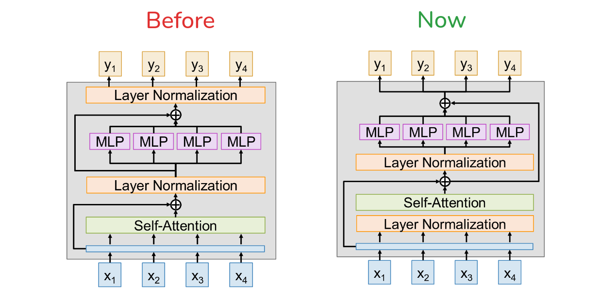
So let’s look at the original architecture from the “Attention is All You Need” paper, which is what’s shown here on the left. This is what’s known as a “Post-Norm” Transformer. And it has a kind of weird property if you look closely at the residual connections. The Layer normalization step happens outside the residual connection. It happens after you add the output of the self-attention block back to the input. Now, let’s do a little thought experiment. What’s the point of a residual connection? It’s to make it easy for a block to learn an identity function, so that we can stack many layers without performance degrading. So, what if our self-attention block learns to output all zeros? In a standard ResNet, the output of the block would be x + 0 = x. But here, the output is LayerNorm(x + 0), which is just LayerNorm(x). It’s not x. So, this architecture can’t actually learn a true identity function. The signal is always getting re-normalized. This can lead to some instabilities, especially at the beginning of training, as the gradients flowing back through the network can be a bit chaotic.

So, what’s the solution? It’s a simple fix that has become almost standard practice. You just move the layer normalization. Instead of putting it after the addition, you move the layer normalization before the Self-Attention and MLP blocks. So now it’s inside the residual branch. This is called a Pre-Norm Transformer. If the self-attention block outputs all zeros, the output of the entire sub-block is x + SelfAttention(LayerNorm(x)). If the self-attention part is zero, the output is x. It can now learn a perfect identity function. Empirically, this small change has been shown to make training significantly more stable, which is a huge win for these massive-scale models.

Alright, so that’s the first big tweak: move from Post-Norm to Pre-Norm. The next common tweak is to the normalization layer itself. People found that you can simplify Layer Normalization a bit and get even better results. This brings us to RMSNorm, which stands for Root-Mean-Square Normalization. If you recall, standard LayerNorm first subtracts the mean to center the data, and then divides by the standard deviation to scale it. RMSNorm gets rid of the centering step. It only scales the vector by its root-mean-square, as you can see in the formula. It still has a learnable gain parameter \(\gamma\), but it doesn’t have the learnable shift \(\beta\).

\[ \begin{align} y_i &= \frac{x_i}{RMS(x)} \gamma_i \\ RMS(x) &= \sqrt{\varepsilon + \frac{1}{N} \sum_{i=1}^N x_i^2} \end{align} \]

This makes the computation slightly simpler and faster. And for reasons that are still being actively studied, this also tends to make training a bit more stable than the full LayerNorm, especially in the Pre-Norm configuration. So, if you look at the source code of many modern open-source LLMs like Llama, you will find they use this exact Pre-Norm architecture with RMSNorm

Okay, so we’ve tweaked the normalization. The next common place for tweaks is inside that other part of the block, the feed-forward MLP. The classic MLP used in the original Transformer is a very simple two-layer feed-forward network. You take your input X of dimension [N x D] project it up to a wider dimension, typically 4D using W₁ [D x 4D] and W₂ [4D x D], apply a non-linearity like ReLU, and then project it back down to D

\[ \underbrace{Y}_{N \times D} = \max(0, XW_1)W_2 \]

Very straightforward. But it turns out there are other ways to design this MLP block that work a bit better. A very popular variant today is called the SwiGLU MLP. Instead of one big projection up, we now have two separate linear projections, W₁ and W₂, [D x H]. The output of the first projection, XW₁, is passed through a Swish activation function \(\sigma\). The output of the second projection, XW₂, is not passed through an activation. We then take these two results and multiply them together element-wise. This is the “gating” part of the Gated Linear Unit, or GLU. Finally, that gated result is passed through a third projection matrix, W₃ [H x D] to get the final output.

\[ Y = (\sigma(XW_1) \odot XW_2)W_3 \]

It’s a more complex interaction, but empirically, it just works better. To keep the number of parameters roughly the same as the classic MLP, you can set the intermediate dimension H to be 8D/3. Again, many modern LLMs like Llama use this exact SwiGLU formulation.

Now, you might ask, why does this work better? What’s the deep theoretical reason for this specific combination of projections and gating? And this is one of those moments where, as a researcher, I have to be very honest with you. The paper that introduced this, “GLU Variants Improve Transformers,” has this wonderfully candid line

“We offer no explanation as to why these architectures seem to work; we attribute their success, as all else, to divine benevolence.”

And I think that’s a perfect encapsulation of a lot of deep learning research. We have some high-level intuitions—gating lets the network control information flow more dynamically—but often, these specific architectural choices are found through extensive empirical exploration. We try a bunch of things, and some just work better than others, and then we try to understand why after the fact. It’s a testament to the fact that this is still very much an empirical science.

Okay, that brings us to the final, and perhaps most impactful, tweak to the modern Transformer architecture: the Mixture of Experts, or MoE introduced in paper “Outrageously Large Neural Networks: The Sparsely-Gated Mixture-of-Experts Layer” by Shazeer et al, in 2017. This is a really big idea. We’ve talked about how these models have scaled up to hundreds of billions or even trillions of parameters. A major problem with that is that for every single input token, you have to do a matrix multiplication with all of those weights. The computational cost grows with the parameter count. The idea behind MoE is to decouple the number of parameters from the amount of compute. What if, instead of having one giant MLP in each block, we have E separate sets of MLP weights? Each of these MLPs is called an “expert.”

Here’s how it works. For each token that enters the MoE layer, we use a small, learnable “router” network to decide which of the E experts are most relevant for processing this specific token. The router predicts a probability distribution over the experts, and we then route the token to be processed by only a small number, A, of the top-scoring experts (where A is much smaller than E). These are the active experts. This is a breakthrough because it means we can have a model with a massive number of parameters (by having many experts, E), but the computational cost for any given token only depends on the small number of active experts, A. It massively increases the parameter count without a proportional increase in compute. It allows for specialization, where different experts can learn to handle different types of inputs.

And this MoE architecture is no longer a niche research idea. All of the biggest LLMs today GPT-4o, Claude 3.7, Gemini 2.5 Pro, all of them, almost certainly use some form of Mixture of Experts. This is how they are able to claim parameter counts in the trillions while still being trainable and runnable. The exact details are usually kept secret, but the general principle of sparse, conditional computation via MoE is the key enabling technology for the current generation of frontier models.